Hunt versus headroom

Rob Calvert Jump and Jo Michell

Just over a year ago, ahead of Jeremy Hunt’s first Autumn Statement, we published a report on how UK public finances are managed and discussed. At the time, the media was awash with claims of a ‘black hole’ in the public finances. We pointed out that this was incoherent because the so-called black hole was nothing more than the difference between an arbitrary fiscal rule and an uncertain forecast.

We also pointed out that forecasts of public debt are highly sensitive to the assumed path of variables such as nominal GDP growth. The latest Autumn Statement and its accompanying OBR projections provide a case in point.

In the run up to the Statement, the media focus had switched from black holes to ‘fiscal headroom‘. This was reported to be around £20bn, and is a measure of the size of the fall in the public debt in the fifth year of the OBR’s forecast – a ‘black hole’ with the sign reversed.

The figure below shows the last three forecasts of public debt from the OBR, along with the historical data published at the time of the forecast. Since the Autumn Statement a year ago, the level of public debt in the final year of the forecasts has fallen from 97.3% of GDP in the November 2022 forecast, to 92.8% of GDP in the most recent one. This forecast revision amounts to nearly £150bn of 2028-29 GDP.

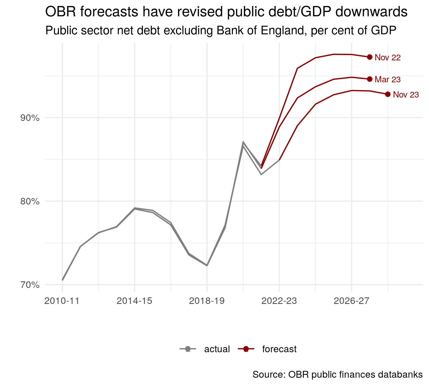
Is this £150bn improvement in the forecast the result of policy actions taken by the government? And if so, why is all the talk of £20bn of headroom, rather than £150bn? The answer to the first question is a firm ‘no’. These shifts in the forecast have nothing to do with policy, and are driven entirely by data revisions and changes in the OBR’s macroeconomic forecasts.

Recent revisions to GDP have shown a stronger recovery from the pandemic than previously thought, alongside higher than expected inflation. As a result, nominal GDP is substantially higher than it was a year ago, and so the debt to GDP ratio is lower.

In the space of a year, data revisions and revised expectations about inflation have, therefore, swamped any change in the debt level driven by policy. Shifts in the positions of the series are far greater than the marginal change between the final two data points – the so-called ‘headroom’ which receives so much attention.

What about the second question? Why are we not talking about £150bn of headroom? The answer to this is unclear, but it is probably the case that the Chancellor of the Exchequer is not actively considering every possible trajectory for the public debt that satisfies his fiscal rules. If he did so, he could substantially increase public spending in a manner that would leave debt falling, as a percentage of GDP, by the end of the OBR’s forecast period.

Consider, for example, the OBR’s November 2023 forecasts for the main fiscal aggregates, displayed in the table below. Public sector net debt, as a percentage of GDP, falls from 93.2% in 2027-28 to 92.8% in 2028-29. Public sector net borrowing is less than 3% of GDP in 2028-29. As a result, the government’s two fiscal targets are met.

year	gdp	gdp_centred	psnd	psnb	gilt_rate	psnd_pct	psnb_pct
2022-23	2552	2650	2251	128.3	3.13	84.94	5.03
2023-24	2726	2761	2458	123.9	4.5	89.03	4.55
2024-25	2798	2841	2603	84.6	4.52	91.62	3.02
2025-26	2887	2938	2724	76.8	4.55	92.72	2.66
2026-27	2995	3051	2845	68.4	4.62	93.25	2.28
2027-28	3106	3162	2947	49.1	4.74	93.2	1.58
2028-29	3218	3274	3039	35.0	4.88	92.82	1.09

OBR forecasts in the November 2023 Economic and Fiscal Outlook.

Now, consider a counterfactual increase in public investment, by £10bn in 2024-25, £15bn in 2025-26, £20bn in 2026-27, £28bn in 2027-28, and then £10bn in 2028-29. This looks something like the Labour Party’s proposed green new deal, in which annual public investment would increase to £28bn over a single parliament. For simplicity we assume multipliers of zero and no impact on inflation, so that nominal GDP is unchanged from the OBR forecasts.

How would this affect public sector borrowing? In 2024-25, it would increase (relative to the OBR’s baseline forecast in table 1) by £10bn. In 2025-26 it would increase by £15bn plus interest payments on the previous year’s £10bn. In 2026-27 it would increase by a further £20bn, plus interest payments on the previous two years’ borrowing, and so on. The resulting time paths for borrowing and debt are displayed in table 2, below.

year	gdp	gdp_centred	psnd	psnb	gilt_rate	psnd_pct	psnb_pct
2022-23	2552	2650	2251	128.3	3.13	84.94	5.03
2023-24	2726	2761	2458	123.9	4.5	89.03	4.55
2024-25	2798	2841	2613	94.6	4.52	91.97	3.38
2025-26	2887	2938	2749.46	92.26	4.55	93.58	3.2
2026-27	2995	3051	2891.63	89.58	4.62	94.78	2.99
2027-28	3106	3162	3023.84	79.31	4.74	95.63	2.55
2028-29	3218	3274	3129.59	48.75	4.88	95.59	1.51

Counterfactual government spending path based on OBR forecasts.

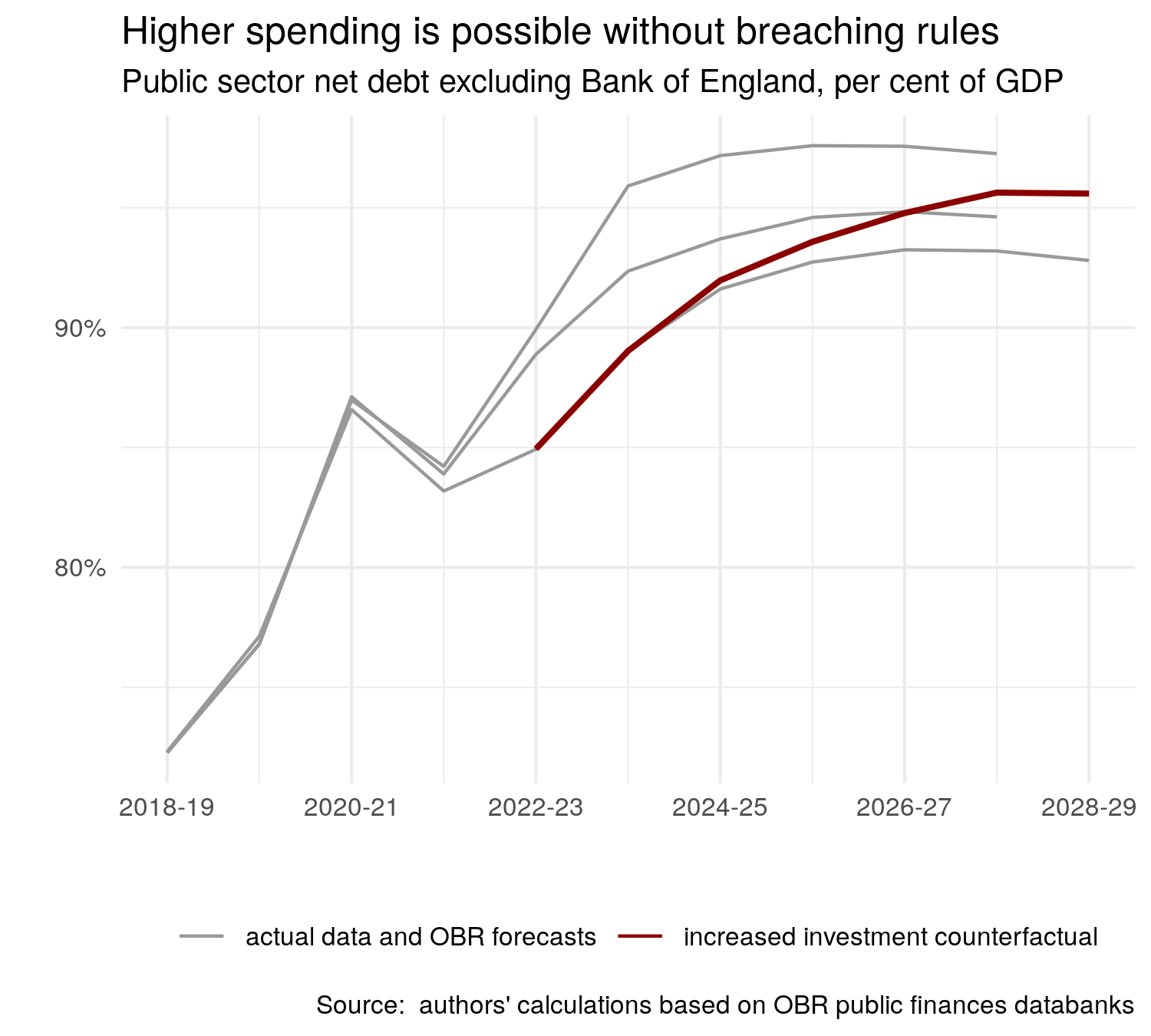
Public sector net debt, as a percentage of GDP, now peaks at a higher level: 95.63% rather than 93.25%. But it is still falling between 2027-28 and 2028-29, and public sector net borrowing is still less than 3% of GDP in 2028-29. As a result, the government’s fiscal targets are still met.

This counterfactual trajectory of debt-to-GDP, alongside the OBR’s recent forecasts are plotted in the figure below. Our counterfactual trajectory is not dissimilar to the OBR’s forecast from March 2023. The end of forecast debt/GDP is around two percentage points of GDP lower than in the November 22 forecast, in which Hunt had defeated the black hole and met his fiscal rules. Given that this was regarded as a success only a year ago, on what basis could our counterfactual trajectory be rejected?

It is clear that ‘headroom’ as reported in the media is not simply a measure of the amount of money that the Chancellor could spend without breaching his fiscal rules. In fact, given its complicated nature, there is no single number that summarises the amount of extra spending consistent with a headline fiscal rule defined by the rate of change of debt-to-GDP at a future point in time. It depends on the distribution of extra spending over the forecast period, as well as the time path of interest rates.

Moreover – and this is, perhaps, more important – it depends on the volatility of the forecasts themselves. The difficulties involved in forecasting economic and fiscal aggregates over a five year horizon is illustrated by pre-budget forecasting exercises published by the Institute of Fiscal Studies and the Resolution Foundation. Their estimates of public debt as a share of GDP at the end of the forecast period differ by nearly 10 percentage points – over £300bn. Minor adjustments to the assumptions that generate these forecasts lead to outcomes an order of magnitude greater than the ‘headroom’ which attracts so much attention.

This is not a rational basis on which to conduct the planning of long-term spending and taxation. It is clear that Hunt’s budget is an exercise in gaming the system. Current nominal tax cuts are ‘paid for’ by creating ‘headroom’ which results from imprecisely specified cuts to government spending towards the end of the forecast period. Moreover, the widely-quoted ‘headroom’ figures have no correspondence whatsoever to the amount of extra money the Chancellor could spend while meeting his rules, and any policy effects are swamped by revisions to the data and forecasts.

As Paul Johnson, head of the Institute for Fiscal studies says, “Aiming for debt to fall in a particular year is not a good fiscal rule”. Simon Wren-Lewis puts it even more bluntly: “falling debt to GDP is a silly rule”.

G7 growth rates and austerity

Rob Calvert Jump and Jo Michell

In August 2022, revisions to official measures of UK output generated headlines because the new figures implied that the economic contraction during the pandemic was greater than previously thought.

At the same time, however, substantial revisions were made to historical data, and these received far less attention. One outcome of these revisions is that the UK’s performance relative to other rich economies during the austerity period of 2010–2016 has been downgraded: growth in real GDP per capita over this period is now meaningfully lower. This means that some recent analyses relying on the older figures are misleading.

For example, in a recent FT article, Chris Giles includes data showing that the UK had the highest growth of real GDP per head in the G7 between 2010 and 2016. Inevitably, the article was circulated by defenders of austerity including Rupert Harrison and Tim Pitt, alongside a claim that the data “shows why the idea austerity has caused our growth problems post-GFC doesn’t stack up. During peak austerity (2010-6) UK had strongest GDP per capita growth in G7”.

The data used by Chris Giles are from the International Monetary Fund’s (IMF) October 2022 World Economic Outlook (WEO), and show average annual growth in real GDP per head of 1.4% in the UK between 2010 and 2016, compared with 1.3% in both Germany and the USA. But the October 2022 WEO uses data from the 2021 Blue Book, which were compiled before the most recent set of revisions were introduced.

The 2021 data imply that total per capita growth between 2010 and 2016 was 8.39% in the UK, compared with 8.36% in Germany and 8.27% in the USA. On these numbers, the UK is indeed the highest, albeit by a margin in the second decimal place: under a billion pounds separates the UK and Germany. (This very slim margin appears larger in the FT chart due to growth rates being annualised and then rounded to 1 decimal place, implying UK growth of 8.7% versus German growth of 8.1%, a difference of 0.6 percentage points rather than the actual difference in the IMF data of 0.03 percentage points.)

However, according to the revised figures, real per capita growth in the UK over this period was only 7.7%: total nominal GDP growth between 2010 and 2016 was revised down by around one percentage point in the 2022 data, culminating in lower cash GDP of around £17 billion by 2016. Smaller adjustments to inflation estimates mean that real GDP growth was revised down by around 0.7 percentage points, from 13.4% to 12.7%. Alongside unchanged population estimates, the result is that official real GDP per capita was revised down by around £340 (in 2019 prices) by 2016 – an amount approximately equal to a third of the average household energy bill in that year.

Chart showing downward revisions to UK nominal GDP growth between 2011 and 2016

These revisions are summarised by the ONS here, and their sources are discussed here. The bulk of the revisions are due to the contribution of the insurance industry to GDP being revised down by the use of Solvency II regulatory data, as well as improvements to the way pension schemes are measured. In addition, and of particular relevance for the current exercise, part of the revisions are due to the ONS, “bringing through a package of sources and methods changes that improve the international comparability of the UK gross domestic product (GDP) estimates.”

These revisions make a material difference to UK GDP, as well as its international ranking. On the basis of the latest official figures taken directly from national statistical agencies, real UK per capita growth of 7.7% during the austerity period compares with 8.4% for Germany and 8.2% for the US.

Chart comparing growth rates in US, UK and Germany between 2010 and 2016.

So, based on the most recent data, the UK did not have the fastest growth in GDP per capita between 2010 and 2016.

Aside from this, as others have noted, focusing narrowly on the 2010-2016 period is potentially misleading. When austerity was implemented, the UK was in the process of recovering from the 2008 recession. It is likely that there was substantial spare capacity which, under strong demand conditions, could have been quickly reabsorbed into economic activity. If we start our comparison at the pre-crisis peak (2007 for the UK and US, 2008 for Germany), rather than 2010, the divergence is much greater: by 2016, real UK GDP per capita had increased by 2.8% on its pre-crisis level, compared with 5.5% for the US and 7.1% for Germany. Much of UK growth during between 2010 and 2016 was recovering losses from the recession: GDP per capita did not reach pre-2008 levels until 2014, compared to 2011 for Germany and 2012 for the US.

As Chris Giles notes, “Most economists now accept that the sharp reductions in public spending between 2010 and 2015 delayed the recovery from the financial crisis”. Comparing outcomes with pre-crisis levels is not, therefore, “baseline bingo” as claimed by Rupert Harrison. These outcomes are hard to square with Harrison’s claim that this is “what catch up looks like”.

Chart showing real GDP per capita between 2007 and 2016 in US, UK and Germany

These data revisions highlight the dangers in drawing strong conclusions – particularly about politically loaded topics – from small differences in data that are subject to measurement error and revision. It is inevitable that an FT article claiming that UK growth per head was highest in the G7 during the main austerity years will be used as justification for austerity policies. But, on the basis of the most recent and accurate data available, the claim is false. UK GDP growth was relatively strong by international standards (and may yet be revised back to the top of the table) but this statement ought to be placed in its proper context, using a variety of data sources and an understanding of their strengths and weaknesses.

	Nominal GDP (YBHA)		Real GDP (ABMI)
Year	2021 Blue Book	2022 Blue Book	2021 Blue Book	2022 Blue Book	IMF 2022 WEO
2010	1,612,195	1,612,381	1,884,515	1,876,058	1,884,515
2011	1,669,509	1,664,211	1,911,983	1,896,087	1,911,983
2012	1,721,355	1,713,241	1,940,087	1,923,551	1,940,087
2013	1,793,155	1,782,296	1,976,755	1,958,557	1,976,755
2014	1,876,162	1,862,827	2,035,883	2,021,225	2,035,883
2015	1,935,212	1,920,998	2,089,276	2,069,595	2,089,276
2016	2,016,638	1,999,461	2,136,566	2,114,406	2,136,566

Data are in millions of pounds (2019 pounds for the real data). Data downloaded from ONS and IMF websites on 20th March 2023. Note that the 2022 Blue Book dataset was only published on the 31st October 2022, too late for inclusion in the IMF’s October 2022 World Economic Outlook. The revisions were initially introduced (and reported on) in August 2022, the quarter before the Blue Book publication.

Pension funds and liquidity spirals

Bruno Bonizzi and Jennifer Churchill

Falling prices in UK government bond (aka gilts) markets yesterday forced the Bank of England to intervene: “a material risk to financial stability” led the Bank to “carry out temporary purchases of long-dated UK government bonds” and to postpone the beginning of Quantitative Tapering, i.e. the sale of bond holdings accumulated over the past decade.

Falls in gilt prices are caused by both global factors – the strong dollar and rising global interest rates – and the large unfunded tax cuts announced in Kwasi Kwarteng’s budget. The most immediate worry is the risk of pension funds “falling over”. How do increasing bond yields pose a problem for pension funds?

Pension funds are widely assumed to function as large passive “containers” of long-term assets which engage in little short-term activity. This is incorrect: pension funds, especially large and mature ones, are sophisticated investors that use leverage and derivatives to achieve their financial objectives.

One such objective, for Defined Benefits (DB) pension funds (that still hold most UK pension fund assets), is best captured by the rise of the Liability Driven Investment (LDI) paradigm. According to LDI, the ultimate goal of pension funds is not the maximisation of returns per se, but performance against the commitments originating from pension liabilities. The key objective of LDI is the minimisation and stabilisation of the so-called “funding deficit”, the difference between the market value of assets and the discounted value of the future pensions to be paid (liabilities).

To achieve the stabilisation of the “funding deficit”, pension funds use a dedicated protection or liability-matching portfolio. This involves strategies that makes the value of assets move in the same direction as the valuation of liabilities. The most important influence on the funding deficit is movements in interest rates: if rates fall, the value of liabilities rises because bond yields are used as discount rates. But if pension funds invest in bonds with similar duration (i.e. sensitivity to interest rate changes) to their liabilities, their assets will also increase by a similar amount, leaving the funding deficit unchanged.

As well as bonds, these strategies also use interest rate swaps, which act in a similar way: pension funds pay a variable rate (e.g. the LIBOR or its recent replacement SONIA) in exchange for a fixed interest payment (the swap rate). By so doing they hedge against interest rate changes. Another LDI strategy is to use repos: pension funds can use their gilts to borrow in the repo market, and then buy more gilts, effectively doubling their exposure to gilts, and thus the degree of interest rate hedging.

The advantage of using repos and derivatives is that it frees up space to invest in other assets. Rather than fully investing their portfolio in bonds, pension funds typically hold a growth portfolio which is invested in all sorts of higher-risk assets, with the objective of increasing returns. This too can make use of derivatives, especially to hedge foreign currency risk. Data from the the ONS Financial Survey of Pension Schemes shows that interest rate swaps and foreign exchange forwards account for almost the totality of derivatives held by pension funds, and these sum (in gross terms) to over 10% of the value of their assets. And while LDI is only relevant to DB pension funds with debt-like liabilitiesall pension funds hedge their overseas assets.

These strategies all require collateral, often short-term bonds. A decline in the market value of collateral or the value of the derivative contracts can lead to margin calls on repo or on interest rate swaps, as explained by Toby Nangle. Similarly, if the value of the sterling falls, pension funds might face margin calls on their foreign exchange derivative positions.

This means that pressure in the short-term bond market can spill over into the market for long-term bonds. To meet margin calls, pension funds can be forced at the extreme to sell growth assets (such as equity, or long-term bonds) to raise the required liquidity to meet margin calls. This is what was seen in the wake of the budget, with pension fund managers reportedly “throwing the kitchen sink to meet margin calls”. If margin calls are not met then collateral could be seized and liquidated, further adding to the downward pressure on asset prices.

This is how we find ourselves in liquidity spiral territory – a situation of severe financial instability, as markets become one-sided, depressing asset prices and potentially provoking more margin calls. The risk of such instability lay behind the decision by the BoE to intervene.

More trouble could be on the horizon: similar liquidity spirals could originate in other derivative markets, such as foreign exchange derivatives as the Pound keeps depreciating against the dollar, or other financial institutions. The possibility of a broader “dash for cash”, requiring more BoE intervention, is still very much on the cards.

Do economists need to talk about consumption?

Chart showing measures of CO2 emissions for high-income countries

This post was originally published here, as part of a series titled Demanding change by changing demand produced by environmental charity Global Action Plan. Some similar themes are explored in more technical detail in the context of lower- and middle- income countries in a recent working paper for the ILO, co-authored with Adam Aboobaker.

For much of the last thirty years or so, progressive economists have argued that macroeconomic policy is too tight. In simpler terms, this means that some combination of higher government spending, lower taxation, and lower interest rates will lead to more jobs and higher incomes.

Such arguments are sometimes presented as part of advocacy for initiatives responding to the environmental crisis, such as the Green New Deal. For the most part, however, the environmental implications of higher near-term economic activity in rich countries do not attract much attention – it is taken as given that higher economic activity, as measured by gross domestic product (GDP), is unequivocally positive.

The current situation of high inflation, driven by energy shortages, war and climate change, serves as a sharp reminder that there is something missing in analysis which sees higher growth as an entirely free lunch. Almost all economic activity depletes scarce physical resources and generates carbon emissions. Higher employment usually comes at the cost of higher emissions. Furthermore, it is possible that we are now also reaching the end of the historic period in which physical resources were usually immediately available – so that economic activity could quickly rise in response to higher overall spending. The era of the Keynesian free lunch may be ending, replaced by a regime characterised by recurring inflationary episodes.

This puts progressive economists, like myself, who believe that the economies of rich countries are predominantly demand driven – meaning that higher overall spending means more jobs and higher incomes – in an uncomfortable position.

This view relies partly on the idea of the “multiplier”. This is the claim, which is well supported by empirical evidence, that every pound of new spending in the economy will generate additional income and spending over and above the initial pound spent. The mechanism works, to a large extent, by stimulating consumption spending: if a new government investment project is initiated – to provide additional green energy, for example – the money spent on the project – on wages, transport and materials – will be received by individuals and businesses as income. Some of this additional income will be spent on consumption, generating a second round of additional new incomes.

Similarly, the argument that redistribution from those on higher incomes to those on lower incomes is good for growth relies on the fact that those on lower incomes spend a greater proportion of their incomes on consumption goods – redistribution from rich to poor thus raises total consumption expenditure and economic activity.

How are progressive economists to respond to the now inescapable fact that current resource use greatly exceeds planetary limits, and “decoupling” – the trend for energy and resource use per dollar of spending to fall as GDP rises – will not be sufficient to stay within planetary boundaries if steady GDP growth continues?

There is no single answer to this question – the appropriate response will require action on many fronts simultaneously. However, economists are beginning to consider whether we need to introduce constraints on consumption, at least for those on higher incomes in rich countries, as part of the solution. Rather than relying only on voluntary consumer choice and natural shifts in consumption patterns – such as the trend towards lower consumption of meat in some rich countries – it may be that state intervention is required to influence both overall levels of consumption and its distribution.

There are two main arguments in favour of constraining consumption. The first is straightforward: all consumption, whether of food, transport, clothing or shelter, involves carbon emissions and resource depletion. Reduced consumption growth should translate directly into lower emissions growth.

The other relates to the need to reallocate current resources, including labour, towards the investment needed to fundamentally reshape our economic systems. Lower consumption means fewer people working in industries which provide for consumption spending, and fewer raw materials devoted to the production of consumption goods. This frees up resources for green investment: people and materials can be re-deployed towards the investment projects which are urgently needed.

This raises some thorny questions: what policy tools can be used to shift the composition and scale of consumption? Which groups should face incentives – or compulsion – to reduce consumption and what form should these measures take? How will voluntary shifts in consumption interact with more direct measures to reduce consumption? And crucially, how can jobs and incomes be protected without relying on consumption as a key driver of macroeconomic dynamism?

Much of this comes down to issues of distribution. Statistics on poverty make clear that large numbers of people in rich nations are unable to consume sufficient basic necessities. Basic justice dictates that the average incomes and consumption of those in lower income countries be allowed to catch up with those of richer countries. The need for redistribution of income within countries, and income catch-up across countries is undeniable – yet such redistribution, if it were to occur without other changes, will lead to increased overall consumption and emissions.

It is therefore hard to avoid the conclusion that taxation and regulation will be required to limit some part of the energy-intensive consumption of those on higher incomes in rich countries, particularly consumption which can be considered “luxury” consumption.

One plausible response to such suggestions is to claim that voluntary shifts in the kinds of things produced and consumed will naturally lead to reduced emissions, even while “consumption”, as measured by the national accounts, continues to grow. This kind of voluntary behavioural and consumption change – buying fewer cheap clothes, holidaying by rail rather than plane, switching to electric cars – will have a part to play in the transition to a low carbon economy, alongside reorientation from goods consumption to a more services-driven “foundational” economy. It is unlikely, however, that such changes will be sufficient.

The politics of consumption constraints are daunting. Managing competing distributional claims in the face of opposition from increasingly concentrated wealth and power is hard enough when the overall pie is growing. As we move towards a world of potential genuine scarcity, the politics of redistribution will become even more malign. This only emphasises the importance of getting the economics right.

Any successful response to the climate crisis will inevitably involve action and change at all levels – from local organising and “organic” shifts in consumption to reform of financial systems and action to tame corporate power and concentrated wealth. Constraints on the consumption of the relatively well off should be part of such a response. A debate about the economics and politics of these constraints is overdue.

Fiscal silly season

We are entering fiscal silly season. As the budget approaches, we should brace for impact with breathless reporting of context-free statistics about inflation, interest rates and government debt.

The story is likely to go something like this. Inflation is rising. This raises costs on government debt because some of it (index-linked bonds) pays an interest rate linked to inflation. Costs associated with quantitative easing (QE) will also increase because QE is financed by central bank reserves which pay Bank Rate (the Bank of England’s policy rate of interest). Since inflation is rising the Bank will have to raise interest rates to control it. This will increase the financing costs of QE and the cost of issuing new debt for the Treasury.

The conclusion — sometimes implied, sometimes explicit — is usually some version of “the situation is unsustainable therefore the government will have to make cuts”.

While each part of the story is technically correct in isolation, the overall narrative — debt is out of control and the situation is going to get worse because of inflation — doesn’t stand up to scrutiny.

These stories are rarely presented with sufficient context. Instead, journalists tend to rely on statistical soundbites such as “public debt is the highest since … ”. This is rarely if ever accompanied by the fact that debt/GDP is a fairly meaningless number.

The problems associated with government debt essentially boil down to the fact that debt involves redistribution. In the case of the government this means redistribution in the form of transfers from tax payers to bond holders. This is politically difficult. (This is also why “but currency issuer …” responses to these issues are largely beside the point — the problems of debt management are ultimately political not technical).

The ratio of debt to GDP tells us very little about the current political difficulties arising from debt servicing. Instead, the relevant magnitudes are total interest payments and tax revenues.

Total interest payments are equal to the debt stock multiplied by the effective interest rate on government debt. Focusing on the debt stock in isolation is thus equivalent to representing the area of a rectangle by the length of one side.

A better indicator of the risks associated with public debt is the ratio of government interest payments to tax revenues, as plotted in the figure below.

Interest payments on government debt have indeed risen recently. A spike in June triggered media articles about the highest interest payments on record. In context, such statistics are shown to be meaningless. Interest payment have risen to around 6% of taxation over a four quarter period, compared with all-time lows of about 5.3%. (Calculated on a 12 monthly basis this rises to around 6.5%). It is hard to see signs that the sky is falling.

In fact, this indicator overstates current interest costs. This is because much of the interest paid by the Treasury is paid to the Bank of England which holds a substantial chunk (currently around 37%) of UK government debt as a result of QE (see chart below). Most of this interest is returned directly to the Treasury. Since the start of QE, this has saved the Treasury over £100bn in interest costs.

Adjusting for this reduction in interest payments produces the figure below: net interest payments sum to around 4.7% of tax revenues over the last four quarters (or 5.2% on a rolling 12 monthly basis).

What of the dangers ahead? It is true that if inflation rises, then interest costs will rise, all else equal. But the scale of these rises is not predetermined, and will be affected by policy.

First, persistent inflation is far from a certainty. If if inflation does persist in the short term, the Bank does not need to raise interest rates. Hikes in response to price pressures due to pandemic reopening and supply side bottlenecks will do more harm than good — instead the Bank should wait until the economic recovery is clearly underway. In this context, interest rate increases would likely be a good sign, and would be offset by rising tax revenues. Further, the Bank could introduce a “tiered reserve” system which would serve to hold down the rate paid on a substantial proportion of outstanding debt. Short term and index-linked debt can be rolled over at longer maturities, delaying the point at which higher rates would feed into higher interest payments.

In summary, simple claims such as “a one percentage point rise in interest rates and inflation could cost the Treasury about £25bn a year” are not useful without context and explanation of the long list of assumptions required to produce such a figure. The policy conclusions derived from such claims should be taken with a large pinch of salt.

Season’s Greetings and enjoy the festive period!

Loanable funds is not helping

Noah Smith has a Christmas post in which he intervenes in the debate over whether $600 government cheques should be given to rich people or poor people. This is the latest iteration of the age-old debate that stems from the dubious argument that income inequality is good because rich people use resources efficiently and poor people waste them. Noah correctly concludes that this argument is wrong and that cheques should be sent to those on lower incomes. But his argument contains several mistakes.

National Saving

Noah starts by discussing whether the rich or poor are more likely to save their $600 cheque, noting that although the rich have a higher propensity to save than the poor, the effect on “national saving” of windfall gains like a one-off cheque may be hard to predict: “if you want to increase national saving, you might want to give the $600 to Tiny Tim instead of to Scrooge!”

Noah’s assumption, at this point in the argument, is that unspent government cheques will increase “national saving”. Is this plausible?

The official definition of “national saving” is total income, Y, less total consumption expenditure, C, (including government consumption). Since “saving” for each sector is sector income less sector consumption, “national saving” is also equal to private saving plus public saving. Manipulation of accounting definitions demonstrates that S = I + CA, where S is national saving, I is total investment (private and public) and CA is the current account surplus. For a closed economy, CA = 0 and S = I. For “national saving” to increase, either I or CA must increase.

Why would members of the public — rich or poor — depositing government cheques at banks increase national saving?

If the cheques are bond-financed, then private sector financial investors have handed over deposits in return for government bonds, while households have accepted deposits. The overall effect is an increase in bond holdings by the private sector, and a redistribution of private deposit holdings. Since private sector income has increased but consumption has not, private sector saving has increased.

But public sector saving has decreased by an equal amount. National saving is unchanged — as is total income. (The same is true for tax-financed cheques.)

Loanable funds

Noah then poses the question “do we really want to increase national saving?”

On a charitable reading, we can assume that, by “national saving”, Noah means “private sector saving”, and his question should be read accordingly.

To answer the question, Noah uses the loanable funds model. Before going on, we need a brief recap on why this model is incoherent, at least when used without care.

As already noted, S = Y – C = I + CA: “National saving” is just another way of saying “investment plus the current account”. There is no such thing as a “supply of savings”: households can choose to consume or not consume. They cannot decide on the size of S, because it equals Y – C. Households choose C but not Y, therefore they don’t choose S. A macro model which has “supply of saving” as an independent aggregate variable is incorrectly specified.

Noah uses this model to consider what happens when the “supply of saving” increases (which he apparently takes as equivalent to the “supply of” what he calls national saving).

He starts by noting that the usual configuration is such that an increase in the “supply of saving” causes “interest rates or stock returns or whatever” to fall and this in turn raises business investment. He then adjusts the model by asserting, “OK, suppose that the amount of business investment just doesn’t depend much on the rate of return”. (By “rate of return” he means “interest rates or stock returns or whatever”, i.e. the rate paid on loans by business, not the rate of profit on business investment.) This gives a diagram like so:

Now, here comes the punchline:

OK, now suppose that in this sort of world, you give someone $600 and they stick it in the bank. That increases the supply of savings. But it doesn’t do anything to the demand for business investment. Businesses invest the same amount. And the rate of return just goes down … in fact total saving doesn’t even go up!

What’s going on here? The supply of savings has increased yet total saving doesn’t change? To understand what Noah thinks he’s saying, let’s switch to apples briefly. Imagine the same supply-demand diagram as above with a vertical (inelastic) demand curve but this time for apples.

This model says that, assuming the quantity of apples consumed is fixed, if the cost of production of apples decreases (because that’s what the supply curve represents, at least in a competitive market), then the price of apples falls. A similar outcome arises if, instead of the cost of production falling, a magician appears, waves a wand, and a stack of extra apples magically appear all harvested and ready for market. At the marketplace, if nobody knows about the wizard, it just looks like the price of apples has fallen.

This is what Noah is doing with the “increase in supply of savings (apples)” arising from the $600 cheques (magic apples): since the “demand for savings” (apples) is fixed, apple sales (business investment/”national savings”) won’t change, but the price (“the rate of return on stocks or whatever”) falls. On the diagram, it looks like this:

This is incoherent in its own terms because, as already noted, a “supply of savings” doesn’t exist in the same way that a supply of apples does: apples are not one number minus another number.

But even putting this non-trivial issue aside, There is a another problem.

Where did the apples go?

Remember that the “supply of savings” has increased in the sense that the price per unit has fallen. But the actual quantity of “savings” is unchanged, according to Noah.

In apple world, the way this works is that when the magic apples appear, the orchard people, understanding the inelastic demand curve of the marketplace, save themselves some effort, harvest less apples, but take the right amount to the marketplace.

How does it work for the “supply of savings?” Don’t worry, Noah has an answer!

You give the $600 to one person, they stick it in the bank or in the markets, that lowers interest rates or stock returns or whatever, and then other people save $600 less as a result. No change.

Pretty neat. Every time someone banks a $600 cheque, another person responds by spending exactly $600 on consumption! In the aggregate, Noah tells us, every dollar is spent! It’s actually impossible for the private sector to save their cheques!

Conclusion

This kind of incoherence is where you end up when you read results from pairs of lines that do not represent the thing that you are trying to understand. The conclusion that total consumption expenditure increases by an amount exactly equal to the total value of the cheques arises as the result of a sequence of ill-defined concepts and inappropriate assumptions, all bolted together without much thought.

In reality, what will happen is the following. Some cheques will be saved, some will be spent on consumption. Those that are saved will have no effect on national saving and probably little effect on the rate of interest, although they might nudge asset prices up a bit. Higher consumption will lead to higher national income, employment and imports. National income will probably rise by more than the amount spent on consumption because of the multiplier. “National saving” is a residual — income less consumption — and is a priori indeterminate. None of this requires us to go anywhere near a loanable funds model.

Loose use of terminology and hand-waving at poorly-defined graphical models does not constitute macroeconomic analysis.

How pension funds shape financialisation in emerging economies in Colombia and Peru

Guest post: Bruno Bonizzi, Jennifer Churchill and Diego Guevara

In early spring 2020 emerging economies (EEs) were hit by the largest ever episode of portfolio outflows. Stock and bonds were sold as investors fled to safer investments in Europe and the United States, showing once again the fragile nature of EEs’ financial integration. To overcome this problem, one suggested solution is to allow for a larger base of domestic institutional investors, such as pension funds, which can stabilise financial markets. While having a large institutional investor base can be a source of demand for domestic financial securities, it is important to review the evidence from the experience of those EEs where pension funds have existed for more than two decades.

As we show in our forthcoming article, the experience of Colombia and Peru can be instructive. Their pension system, while maintaining a significant parallel public Pay-As-You-Go structure, has a sizeable funded private component with assets that have grown to over 20% of GDP. These were established as part of the Washington Consensus reforms in the 1990s, following the prior example of Chile.

However, more than two decades since the creation of private pension funds, capital markets in the two countries, as in the rest of Latin America, remain small and underdeveloped. It is perhaps for this reason that the experience of pension funds in Latin America remains under-researched by financialisation scholarship. However, recent literature has put forward the idea that financialisation patterns, while having common tendencies, can present “variegated” forms. Pension funds play a role in this process by exerting an important role in shaping the demand for financial assets, even if this does not occur, as in typical “Liberal Market Economies” by fuelling domestic capital markets.

Some key characteristics of Colombia and Peru’s political economy have acted as the distinct determinants of pension fund demand for assets, shaping a specific form of financialisation. Firstly, pension funds in these countries reflect the characteristics of Hierarchical Market Economies, the Latin American variety of capitalism. Workers and unions have very limited control over how pension fund assets are invested, as pension funds are provided by private companies as pure individual retirement accounts. Investment policy is therefore heavily shaped by the interest of the financial industry, which was also key in promoting their establishment and in shaping their regulation since.

But next to these considerations, pension fund asset demand in Colombia and Peru has been structurally constrained by the limited by limited effective space in domestic capital markets. These two countries have a highly “extraverted” growth regime, where commodity exports play a key role in determining aggregate demand. As a result of the 2000-2014 commodity price boom, companies had substantial financing coming from export proceeds and foreign direct investment, therefore limiting their issuance of securities in domestic capital markets. Governments too limited their net borrowing during this period, thanks to booming revenues and limited increases in public spending. Additionally, the countries have attracted considerable interest by foreign financial investors, whose weight in domestic bond and stock markets increased. These characteristics reflect the status of Colombia and Peru of as subordinate emerging economies in global financial markets.

Pension funds in Colombia and Peru have looked for other investments. Supported once again by the domestic and international financial industry, these have been found in “alternative assets”, most typically private equity, infrastructure and real-estate funds, as well as in foreign investment, which now account for more than a third and more than 40% of total assets in Colombia and Peru respectively. The latter have been important in stimulating a derivative market to hedge foreign currency positions, mostly vis-á-vis US dollars.

Therefore, pension funds have been important in shaping the financialisation trajectory in these two countries, despite the limited development of domestic capital markets. This can serve as an important lesson to calls for the promotion of private pensions to stabilise capital markets. In emerging economies subject to subordinate forms of economic and financial integration, and where the interests represented are those of a highly concentrated financial industry, pension funds may fail to act as catalysts for deep, liquid and stable domestic capital markets. They may instead contribute to finance privatised forms of infrastructure and real estate and reinforce the hierarchies of global finance.

Three myths about EU’s economic response to the COVID19 pandemic

Daniela Gabor

On Monday 15th, 2020, I took part in the Public Hearing on COVID19 responses at the European Parliament’s ECON committee. This is the text of my introductory remarks.

The COVID19 pandemic confronted EU members with symmetric shocks and profound deflationary forces. In response, governments are running large budget deficits. Their borrowing costs remain low because central banks have acted as public guarantors of confidence.

I would like to unpack three myths about the COVID19 response in Europe.

Myth 1: central banks have overstepped their mandate with disproportionate interventions in government bond markets, undermining fiscal rules.

This argument, as expressed in the Karlsruhe ruling, implies that it is imperative to return to the pre-crisis status quo: a division of macroeconomic labor whereby the ECB targets price-stability, whereas Member States conduct fiscal and economic policies in a manner consistent with European rules.

Through a macro-financial lens, this argument is simply wrong. If we ask how private financial structure and macroeconomic policies interact*, it becomes clear that evolutionary changes in European finance have joined monetary and fiscal policies at the hip. The pre-crisis division of macroeconomic labor is a fiction that we can no longer afford to sustain.

Consider the largest money market for European banks and institutional investors, the €7 trillion repo market. Two out of three euro borrowed through repos use sovereign bonds issued by euro-area members (Germany and Italy the largest) as collateral. Private credit creation —the bread and butter of the ECB’s operations —fundamentally relies on sovereign bonds, and so on fiscal policy. Higher sovereign yields make private credit more expensive. In turn, the repo market creates, and can easily destroy, liquidity for governments, influencing their borrowing conditions and, ultimately, fiscal-policy. In the Euroarea, it creates an exorbitant privilege for Germany: in crisis, banks run to German bunds because these preserve access to collateralised funding. This is why leaders of ‘periphery’ euro countries watch the spread to German bunds nervously.

The ECB did not intervene in sovereign-bond markets because it worried about debt sustainability. As President Lagarde noted in the European Parliament hearing in early June, intervention was needed to effectively support private credit creation, and the transmission mechanism of monetary policy. Improvements in financing conditions for governments, much decried in some European circles, are not a policy target but a side effect of the repo-based sovereign debt order that the founders of the Euro put in place.

But the Euro founders did so without appreciating its complex political ramifications, in particular the structural pressures on central banks to intervene in sovereign bond markets. Given the growing public debt/GDP ratios, and the possibility of renewed pressure on vulnerable sovereigns, it is imperative we rethink this order.

For this, we need to update the institutional framework that governs the relationship between central banks and governments. So far, central banks have improvised through unconventional policy measures, but on terms that they control. In so doing, they entrench a democratic deficit that encourages anti-European sentiment. In the Euroarea, monetary union needs to be accompanied by fiscal union not on grounds of ‘solidarity’, but because the alternative is a disorderly exit from the Euro, particularly if the chorus demanding post-pandemic austerity becomes stronger.

Myth 2 Europe has well-functioning institutions – like the ESM – to provide a safety net for sovereigns in times of crisis.

The Almunia Report on the EFSF/ESM programmes in Greece highlights serious weakness in the institutional mechanisms for backstopping Member States in times of crisis. The ESM put excessive emphasis on fiscal consolidation, with significant social costs for Greek citizens, lacked strategic objectives and prioritized the interests of ESM members over those of Greece. Harsh and counterproductive conditionality for sovereigns stands in clear contrast to the generous support for private finance, as for instance extended by the ECB.

Even if the Almunia recommendations would be enacted in a timely fashion, a reformed ESM can at best alleviate some of the burden of higher public debt. It cannot effectively respond to the cyclical liquidity pressures created by the financial structure described above, particularly as public debt burdens grow across Europe. Equally important, it would not create the fiscal space necessary for Member States to respond counter-cyclically to shocks, and to prioritize green public investments, including public health infrastructure.

This is why the European Commission’s plans for grants under the EU Next Generation are an important first step towards creating an effective European response. But are these enough.

Myth 3 The pandemic recovery plans of the European Commission are ambitious enough.

Bruegel estimates that only a quarter from the grants envisaged in the Next Generation EU will be spent over 2020-2022**. National fiscal policies will have to shoulder the burden of recovery. The EU can and should be more ambitious, prioritizing a green recovery.

It is encouraging that the Commission has reaffirmed its intentions to reserve 25% of EU spending for climate-friendly expenditure. Its efforts should be amplified by pre-crisis commitments to green central banks and to promote sustainable finance in Europe.

Take the ECB. Its support to market actors comes without environmental, tax- or payout-related conditionality. In practice, the ECB continues to subsidise high-carbon activities, and in doing so, it reinforces climate-related risks to financial stability. Its objectives can be recalibrated within the existing treaty framework, as follows***:

The ECB should start to love ‘brown inflation’. In its current version, the Harmonised Index of Consumer Prices ignores the carbon footprint of goods and services. Greening the HICP would take the bite out of the price-stability mandate, while rendering it more consistent with the ECB’s secondary objective.
The ECB should green its monetary policy operations, by removing the preferential treatment to brown assets, and where it judges necessary, by promoting green financial instruments. These two measures should go hand in hand to avoid greenwashing, and would constitute an effective measure to reorient private finance towards sustainable activities.
The Euroarea should institute an open and recurrent process at the highest political level to specify which ‘general economic policies in the Union’ the ECB is required to support. Article 11 of the Treaty on the Functioning of the European Union already mandates ‘environmental protection’. Specifying such protection in relation to the full portfolio of central-bank activities—considerably broader than monetary policy proper—would provide political legitimacy for an unconditional ECB backstop of green public investment. This circular arrangement would amount to a substantial gain in fiscal sovereignty in the euro area.

In parallel, the European Commission, with support from the European Parliament, should accelerate its work on the Renewed Sustainable Finance strategy. A well-defined taxonomy for green and brown activities, and prudential measures guided by the taxonomy, would ensure that private financing of brown activities does not undermine the public investments in the green recovery.

Thank you for your time.

——–

* See Gabor, D. (2020) Critical macro-finance: a theoretical lens. Finance and Society 6(1): 45-55.

**See Darvas, Z. (2020) Three-quarters of Next Generation EU payments will have to wait until 2023. https://www.bruegel.org/2020/06/three-quarters-of-next-generation-eu-payments-will-have-to-wait-until-2023/

*** See Braun, B., Gabor, D. and B. Lemoine (2020) Enlarging the ECB mandate for the common good and the planet. Social Europe. https://www.socialeurope.eu/enlarging-the-ecb-mandate-for-the-common-good-and-the-planet

Mercados emergentes precisam de controle de capital para evitar catástrofes financeiras

Traduzida por Carolina Alves.

Todos os países estão atualmente enfrentando a ameaça sem precedentes de uma crise global da saúde, recessão econômica e colapso financeiro, simultaneamente. Mas, ao contrário dos países ricos, os mercados emergentes (EMs) não têm autonomia política necessária para enfrentar essas crises. A hierarquia global de moedas coloca EMs na periferia dos mercados financeiros globais, expondo-os a paradas súbitas de fluxos de capital causadas por gatilhos como a crise COVID-19. Imediato controle de capital, coordenado pelo FMI,è necessário para evitar um desastre financeiro

Em uma crise financeira global, há uma pressa em manter ativos líquidos denominados em moedas seguras, especialmente dólares americanos. Isso permite ricos países responder a crises com as necessárias ferramentas fiscais e monetárias. O oposto é verdadeiro para os EMs. Desde o surto de COVID-19, investidores internacionais retiraram grandes quantias de ativos dos EMs, causando uma depreciação dramática da moeda, especialmente aqueles expostos à queda dos preços das commodities.

Na última década, ampla liquidez global impulsionada por bancos centrais de países ricos, juntamente com a demanda sustentada por ativos líquidos, levou a enormes fluxos de crédito e investimento de capital nos EMs, onde os títulos e as bolsas de valores cresceram por volta de 15 trilhões para 33 trilhões de dólares americanos entre 2008 e 2019. ‘Economias de fronteira’ e EMs corporações emitiram volumes substanciais de dívida em moeda estrangeira. Com o G20 incentivo, os EMs abriram seus mercados de títulos em moeda nacional para investidores internacionais. No que foi denominado a segunda fase da liquidez global, novos instrumentos e instituições financeiras, como fundos internacionais e fundos de investimento abertos negociados em bolsa (ETF), possibilitaram a fácil negociação global de EMs ativos, consolidando a ilusão de liquidez.

Os EMs agora são confrontados com uma parada repentina de capital, pois as condições globais de liquidez apertam e os investidores fogem do risco: a exposição aos EMs continua sendo uma estratégia de alto risco/alto retorno, a ser liquidada em tempo de crises. Consequentemente, os EMs enfrentam severo ajuste macroeconômico exatamente no momento em que todas as ferramentas disponíveis devem ser usadas para combater a crise de saúde pública apresentada pelo COVID-19. Alguns países podem ser forçados a implementar uma política monetária restritiva na tentativa de manter o acesso ao dólar, enquanto a ação fiscal pode ser restringida pelo medo de perder o acesso a mercados globais. É improvável que as reservas cambiais forneçam ‘colchão de segurança’ suficiente em todos os países.

Há uma necessidade urgente de ação para impedir que essa crise chegue a proporções catastróficas nos EMs. Apesar de pedidos de ação de longa data, ainda não existe credor internacional de última instância. Os únicos instrumentos atualmente disponíveis são empréstimos dos FMI e linhas de swap cambial temporárias entre bancos centrais. Os empréstimos do FMI normalmente impõem ajustes fiscais, o que seria desastroso nas condições atuais. Os Fed está pronto para fornecer dólares americanos a um punhado de bancos centrais: entre os EMs, apenas o México pode acessar as linhas de swap do Fed sob as disposições do NAFTA. Durante a crise financeira global de 2009, o acesso foi concedido apenas ao Brasil e à Coréia do Sul. Mas EMs, no G20 e além, são agora muito mais importantes para o económico crescimento mundial. O fracasso deles, ou de um grande quase-soberano tomador de empréstimo, poderia desencadear um contágio significativo.

Nos pedimos uma ação decisiva para restringir os fluxos financeiros atualmente transmitindo a crise aos EMs. Controles de capital devem ser introduzidos para reduzir a fuga de capitais, para reduzir a falta de liquidez causada por sell-offs nos EMs mercados, e para impedir quedas da moeda e preços dos ativos. A implementação deve ser coordenada pelo FMI para evitar estigma e evitar contágio. As linhas de swap cambial devem ser estendidas para incluir EMs, e então garantir o acesso ao dólar americano. Finalmente, concordamos com as recentes medidas fornecendo uma maior provisão de liquidez pelo FMI usando os Direitos de Saque Especiais (DSE) – mas isso deve ocorrer sem a imposição de ajuste fiscal pró-cíclico.

A crise que se desenrola é uma das mais graves na história econômica. Nós deve garantir que os governos possam fazer todo o possível para proteger seus cidadãos. Em nossa economia globalmente integrada, ações coordenadas são necessárias para minimizar as restrições externamente-impostas às economias emergentes, que por sinal enfrentam a tripla ameaça de pandemia, recessão e crise financeira.

Los Países Emergentes Y En Desarrollo Necesitan Controles De Capital Para Prevenir Una Catástrofe Financiera

Una version corta de esta carta fue publicada en Financial Times, el 25 Marzo

2020.

Traducido al español por: Jimena Sierra y Federico Suárez

(con el apoyo de Daniela Gabor y Luis Eslava)

Actualmente, todos los países enfrentan una amenaza sin precedentes. Esta amenaza es tanto el producto de la crisis de salud global, como de sus efectos en términos de recesión económica y colapso financiero. A diferencia de las naciones ricas, sin embargo, los países emergentes y en desarrollo (PED) carecen de la autonomía política necesaria para enfrentar estas crisis. La jerarquía monetaria global coloca a los PED en la periferia de los mercados financieros globales, lo cual los sobreexpone a choques repentinos causados por fenómenos como la crisis del COVID-19. La Reserva Federal de los Estados Unidos ha anunciado que prestaría hasta USD 60 mil millones a los bancos centrales de México, Brasil, Corea del Sur y Singapur. Aunque bien recibidos, esta línea de crédito no es suficiente. Se necesitan controles inmediatos de capital, coordinados por el FMI, para evitar un desastre financiero.

En una crisis financiera global, hay una urgencia por mantener activos líquidos en monedas seguras, especialmente dólares estadounidenses. Los países ricos pueden responder a este reto con las herramientas fiscales y monetarias necesarias. Sin embargo, esto no es posible, para los PED. Desde el estallido de la crisis de COVID-19, los inversionistas internacionales han retirado grandes sumas de los activos de los PED, lo que ha llevado a una depreciación dramática de la moneda en estos países, especialmente en aquellos que están ya sobreexpuestos debido a la caída de los precios de sus commodities.

Durante la última década, la amplia liquidez a nivel global impulsada por los bancos centrales de los países ricos, junto a una demanda sostenida de activos líquidos, ha direccionado enormes flujos de crédito e inversión en acciones hacia los PED, donde los mercados de bonos y acciones crecieron aproximadamente de 15 billones a 33 billones de dólares entre 2008 y 2019. Las ‘economías de frontera‘ y las corporaciones de los PED han emitido cantidades sustanciales de deuda en moneda extranjera. Con el apoyo del G-20, los PED abrieron sus mercados debonos en moneda nacional a inversores internacionales. En el marco de lo que se ha llamado como la segunda fase de liquidez global, los nuevos instrumentos y las nuevas instituciones financieras, como los fondos internacionales y los fondos de inversión cotizados en bolsa (exchange-traded funds (ETFs) eninglés), han facilitado la negociación global de los activos de los PED, dando lugar a una ilusión de liquidez.

Los PED ahora se enfrentan a un choque repentino por el endurecimiento de las condiciones de liquidez global y debido a que los inversores buscan huir del riesgo: la exposición a los PED sigue siendo una estrategia de alto riesgo y alto retorno, que deja de ser tractiva en tiempos de crisis. En consecuencia, los PED se enfrentan hoy a un severo ajuste macroeconómico precisamente en el momento en que todas las herramientas disponibles deben usarse para contrarrestar la crisis de salud pública causada por el COVID-19. De esta manera, algunos países pueden verse obligados a endurecer su política monetaria en un intento por retener el acceso al dólar estadounidense, mientras que las acciones fiscales pueden verse limitadas por el miedo a perder el acceso a los mercados mundiales. Sin embargo, es poco probable, que las reservas de divisas amortigüen de manera suficiente a todos los países. Esto tendría profundas consecuencias para la economía global: los PED, tanto aquellos que están en el G-20 como fuera de este, son hoy en día mucho más importantes de lo que eran hace una década gracias al crecimiento económico y la expansión de los mercados a nivel global. Frente a estos retos, el fracaso de una acción internacional que facilite préstamos soberanos o cuasi-soberano podría desencadenar en un efecto dominó con consecuencias devastadoras a través del planeta.

Existe una necesidad urgente de actuar para evitar que esta crisis alcance proporciones catastróficas en los PED. A pesar de décadas de discusiones y advertencias, todavía no existe un prestamista internacional de última instancia. Los únicos instrumentos disponibles actualmente son los préstamos del FMI y las líneas de intercambio de divisas entre bancos centrales. Sin embargo, los préstamos del FMI suelen imponer ajustes fiscales, lo cual sería desastroso en las condiciones actuales. La Reserva Federal de los Estados Unidos, por otro lado, está lista para proporcionar dólares estadounidenses a un puñado de bancos centrales: el problema es que entre los PED solo México, Corea del Sur y Brasil pueden acceder a estas líneas de intercambio de la Reserva, por un monto de hasta USD 60bn. No obstante, estos acuerdos ad hoc excluyen una gran proporción de las necesidades de los PED de liquidez en dólares.

Debido a lo anterior, hacemos un llamado a tomar acciones decisivas para restringir los flujos financieros que actualmente están transfiriendo la crisis a los mercados emergentes. Deben introducirse controles de capital para restringir la salida repentina de flujos, reducir la falta de liquidez provocada por las ventas generalizadas de activos en los mercados de los PED y detener con esto las caídas de los precios de las monedas y de los activos nacionales. La implementación de las medidas que se adopten debe coordinarse por el FMI para evitar la estigmatización y prevenir un contagio generalizado. Las líneas de intercambio de divisas deben extenderse para incluir más PED, a fin de garantizar el acceso a dólares estadounidenses. Finalmente, coincidimos con los llamados recientes al FMI para proveer una mayor liquidez, utilizando derechos especiales de giro (DEG), sin generar con esto la imposición de ajustes fiscales pro-cíclicos.

La crisis que se esta desarrollando actualmente es una de las más graves en la historia económica. Debemos asegurarnos que los gobiernos puedan hacer todo lo posible para proteger a sus ciudadanos. En nuestra economía global e integrada, se necesita una acción coordinada para minimizar las restricciones impuestas externamente a los países en desarrollo y emergentes, ya que estos se enfrentan hoy a una crisis triple: la pandemia, la recesión económica y una crisis financiera.