G7 growth rates and austerity

Rob Calvert Jump and Jo Michell

In August 2022, revisions to official measures of UK output generated headlines because the new figures implied that the economic contraction during the pandemic was greater than previously thought. 

At the same time, however, substantial revisions were made to historical data, and these received far less attention. One outcome of these revisions is that the UK’s performance relative to other rich economies during the austerity period of 2010–2016 has been downgraded: growth in real GDP per capita over this period is now meaningfully lower. This means that some recent analyses relying on the older figures are misleading.

For example, in a recent FT article, Chris Giles includes data showing that the UK had the highest growth of real GDP per head in the G7 between 2010 and 2016. Inevitably, the article was circulated by defenders of austerity including Rupert Harrison and Tim Pitt, alongside a claim that the data “shows why the idea austerity has caused our growth problems post-GFC doesn’t stack up. During peak austerity (2010-6) UK had strongest GDP per capita growth in G7”.

The data used by Chris Giles are from the International Monetary Fund’s (IMF) October 2022 World Economic Outlook (WEO), and show average annual growth in real GDP per head of 1.4% in the UK between 2010 and 2016, compared with 1.3% in both Germany and the USA. But the October 2022 WEO uses data from the 2021 Blue Book, which were compiled before the most recent set of revisions were introduced.

The 2021 data imply that total per capita growth between 2010 and 2016 was 8.39% in the UK, compared with 8.36% in Germany and 8.27% in the USA. On these numbers, the UK is indeed the highest, albeit by a margin in the second decimal place: under a billion pounds separates the UK and Germany. (This very slim margin appears larger in the FT chart due to growth rates being annualised and then rounded to 1 decimal place, implying UK growth of 8.7% versus German growth of 8.1%, a difference of 0.6 percentage points rather than the actual difference in the IMF data of 0.03 percentage points.)

However, according to the revised figures, real per capita growth in the UK over this period was only 7.7%: total nominal GDP growth between 2010 and 2016 was revised down by around one percentage point in the 2022 data, culminating in lower cash GDP of around £17 billion by 2016.  Smaller adjustments to inflation estimates mean that real GDP growth was revised down by around 0.7 percentage points, from 13.4% to 12.7%. Alongside unchanged population estimates, the result is that official real GDP per capita was revised down by around £340 (in 2019 prices) by 2016 – an amount approximately equal to a third of the average household energy bill in that year.

Chart showing downward revisions to UK nominal GDP growth between 2011 and 2016

These revisions are summarised by the ONS here, and their sources are discussed here. The bulk of the revisions are due to the contribution of the insurance industry to GDP being revised down by the use of Solvency II regulatory data, as well as improvements to the way pension schemes are measured. In addition, and of particular relevance for the current exercise, part of the revisions are due to the ONS, “bringing through a package of sources and methods changes that improve the international comparability of the UK gross domestic product (GDP) estimates.” 

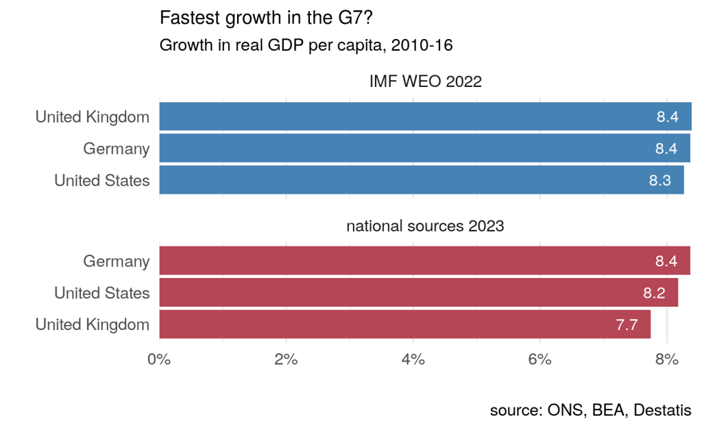
These revisions make a material difference to UK GDP, as well as its international ranking. On the basis of the latest official figures taken directly from national statistical agencies, real UK per capita growth of 7.7% during the austerity period compares with 8.4% for Germany and 8.2% for the US.

Chart comparing growth rates in US, UK and Germany between 2010 and 2016.

So, based on the most recent data, the UK did not have the fastest growth in GDP per capita between 2010 and 2016. 

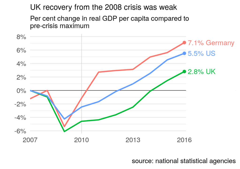
Aside from this, as others have noted, focusing narrowly on the 2010-2016 period is potentially misleading. When austerity was implemented, the UK was in the process of recovering from the 2008 recession. It is likely that there was substantial spare capacity which, under strong demand conditions, could have been quickly reabsorbed into economic activity. If we start our comparison at the pre-crisis peak (2007 for the UK and US, 2008 for Germany), rather than 2010, the divergence is much greater: by 2016, real UK GDP per capita had increased by 2.8% on its pre-crisis level, compared with 5.5% for the US and 7.1% for Germany. Much of UK growth during between 2010 and 2016 was recovering losses from the recession: GDP per capita did not reach pre-2008 levels until 2014, compared to 2011 for Germany and 2012 for the US.

As Chris Giles notes, “Most economists now accept that the sharp reductions in public spending between 2010 and 2015 delayed the recovery from the financial crisis”. Comparing outcomes with pre-crisis levels is not, therefore, “baseline bingo” as claimed by Rupert Harrison. These outcomes are hard to square with Harrison’s claim that this is “what catch up looks like”.

Chart showing real GDP per capita between 2007 and 2016 in US, UK and Germany

These data revisions highlight the dangers in drawing strong conclusions – particularly about politically loaded topics – from small differences in data that are subject to measurement error and revision. It is inevitable that an FT article claiming that UK growth per head was highest in the G7 during the main austerity years will be used as justification for austerity policies. But, on the basis of the most recent and accurate data available, the claim is false. UK GDP growth was relatively strong by international standards (and may yet be revised back to the top of the table) but this statement ought to be placed in its proper context, using a variety of data sources and an understanding of their strengths and weaknesses.

Nominal GDP (YBHA)Real GDP (ABMI)
Year2021 Blue Book2022 Blue Book2021 Blue Book2022 Blue BookIMF 2022 WEO
20101,612,1951,612,3811,884,5151,876,0581,884,515
20111,669,5091,664,2111,911,9831,896,0871,911,983
20121,721,3551,713,2411,940,0871,923,5511,940,087
20131,793,1551,782,2961,976,7551,958,5571,976,755
20141,876,1621,862,8272,035,8832,021,2252,035,883
20151,935,2121,920,9982,089,2762,069,5952,089,276
20162,016,6381,999,4612,136,5662,114,4062,136,566

Data are in millions of pounds (2019 pounds for the real data). Data downloaded from ONS and IMF websites on 20th March 2023. Note that the 2022 Blue Book dataset was only published on the 31st October 2022, too late for inclusion in the IMF’s October 2022 World Economic Outlook. The revisions were initially introduced (and reported on) in August 2022, the quarter before the Blue Book publication.

Loanable funds is not helping

Noah Smith has a Christmas post in which he intervenes in the debate over whether $600 government cheques should be given to rich people or poor people. This is the latest iteration of the age-old debate that stems from the dubious argument that income inequality is good because rich people use resources efficiently and poor people waste them. Noah correctly concludes that this argument is wrong and that cheques should be sent to those on lower incomes. But his argument contains several mistakes.

National Saving

Noah starts by discussing whether the rich or poor are more likely to save their $600 cheque, noting that although the rich have a higher propensity to save than the poor, the effect on “national saving” of windfall gains like a one-off cheque may be hard to predict: “if you want to increase national saving, you might want to give the $600 to Tiny Tim instead of to Scrooge!”

Noah’s assumption, at this point in the argument, is that unspent government cheques will increase “national saving”. Is this plausible?

The official definition of “national saving” is total income, Y, less total consumption expenditure, C, (including government consumption). Since “saving” for each sector is sector income less sector consumption, “national saving” is also equal to private saving plus public saving. Manipulation of accounting definitions demonstrates that S = I + CA, where S is national saving, I is total investment (private and public) and CA is the current account surplus. For a closed economy, CA = 0 and S = I. For “national saving” to increase, either I or CA must increase.

Why would members of the public — rich or poor — depositing government cheques at banks increase national saving?

If the cheques are bond-financed, then private sector financial investors have handed over deposits in return for government bonds, while households have accepted deposits. The overall effect is an increase in bond holdings by the private sector, and a redistribution of private deposit holdings. Since private sector income has increased but consumption has not, private sector saving has increased.

But public sector saving has decreased by an equal amount. National saving is unchanged — as is total income. (The same is true for tax-financed cheques.)

Loanable funds

Noah then poses the question “do we really want to increase national saving?”

On a charitable reading, we can assume that, by “national saving”, Noah means “private sector saving”, and his question should be read accordingly.

To answer the question, Noah uses the loanable funds model. Before going on, we need a brief recap on why this model is incoherent, at least when used without care.

As already noted, S = Y – C = I + CA: “National saving” is just another way of saying “investment plus the current account”. There is no such thing as a “supply of savings”: households can choose to consume or not consume. They cannot decide on the size of S, because it equals Y – C. Households choose C but not Y, therefore they don’t choose S. A macro model which has “supply of saving” as an independent aggregate variable is incorrectly specified.

Noah uses this model to consider what happens when the “supply of saving” increases (which he apparently takes as equivalent to the “supply of” what he calls national saving).

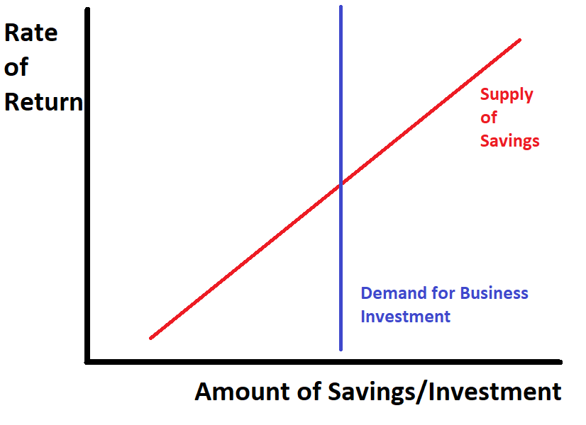
He starts by noting that the usual configuration is such that an increase in the “supply of saving” causes “interest rates or stock returns or whatever” to fall and this in turn raises business investment. He then adjusts the model by asserting, “OK, suppose that the amount of business investment just doesn’t depend much on the rate of return”. (By “rate of return” he means “interest rates or stock returns or whatever”, i.e. the rate paid on loans by business, not the rate of profit on business investment.) This gives a diagram like so:

Now, here comes the punchline:

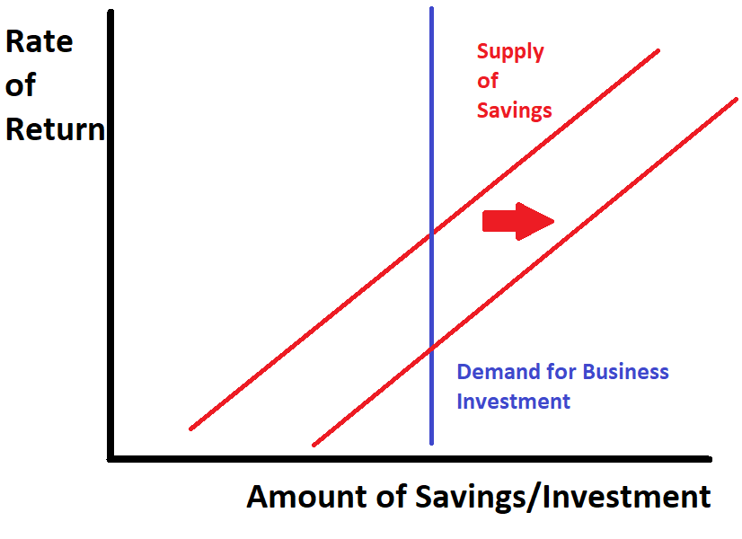
OK, now suppose that in this sort of world, you give someone $600 and they stick it in the bank. That increases the supply of savings. But it doesn’t do anything to the demand for business investment. Businesses invest the same amount. And the rate of return just goes down … in fact total saving doesn’t even go up!

What’s going on here? The supply of savings has increased yet total saving doesn’t change? To understand what Noah thinks he’s saying, let’s switch to apples briefly. Imagine the same supply-demand diagram as above with a vertical (inelastic) demand curve but this time for apples.

This model says that, assuming the quantity of apples consumed is fixed, if the cost of production of apples decreases (because that’s what the supply curve represents, at least in a competitive market), then the price of apples falls. A similar outcome arises if, instead of the cost of production falling, a magician appears, waves a wand, and a stack of extra apples magically appear all harvested and ready for market. At the marketplace, if nobody knows about the wizard, it just looks like the price of apples has fallen.

This is what Noah is doing with the “increase in supply of savings (apples)” arising from the $600 cheques (magic apples): since the “demand for savings” (apples) is fixed, apple sales (business investment/”national savings”) won’t change, but the price (“the rate of return on stocks or whatever”) falls. On the diagram, it looks like this:

This is incoherent in its own terms because, as already noted, a “supply of savings” doesn’t exist in the same way that a supply of apples does: apples are not one number minus another number.

But even putting this non-trivial issue aside, There is a another problem.

Where did the apples go?

Remember that the “supply of savings” has increased in the sense that the price per unit has fallen. But the actual quantity of “savings” is unchanged, according to Noah.

In apple world, the way this works is that when the magic apples appear, the orchard people, understanding the inelastic demand curve of the marketplace, save themselves some effort, harvest less apples, but take the right amount to the marketplace.

How does it work for the “supply of savings?” Don’t worry, Noah has an answer!

You give the $600 to one person, they stick it in the bank or in the markets, that lowers interest rates or stock returns or whatever, and then other people save $600 less as a result. No change.

Pretty neat. Every time someone banks a $600 cheque, another person responds by spending exactly $600 on consumption! In the aggregate, Noah tells us, every dollar is spent! It’s actually impossible for the private sector to save their cheques!

Conclusion

This kind of incoherence is where you end up when you read results from pairs of lines that do not represent the thing that you are trying to understand. The conclusion that total consumption expenditure increases by an amount exactly equal to the total value of the cheques arises as the result of a sequence of ill-defined concepts and inappropriate assumptions, all bolted together without much thought.

In reality, what will happen is the following. Some cheques will be saved, some will be spent on consumption. Those that are saved will have no effect on national saving and probably little effect on the rate of interest, although they might nudge asset prices up a bit. Higher consumption will lead to higher national income, employment and imports. National income will probably rise by more than the amount spent on consumption because of the multiplier. “National saving” is a residual — income less consumption — and is a priori indeterminate. None of this requires us to go anywhere near a loanable funds model.

Loose use of terminology and hand-waving at poorly-defined graphical models does not constitute macroeconomic analysis.

Developing and emerging countries need capital controls to prevent financial catastrophe

A shorter version of this letter was published in the Financial Times on 25 March 2020.

All countries currently face the unprecedented threat of a simultaneous and global health crisis, economic recession and financial meltdown. But unlike rich nations, emerging and developing countries  (DECs) lack the policy autonomy needed to confront these crises. The global currency hierarchy places DECs in the periphery of global financial markets, exposing them to sudden stops caused by triggers such as the COVID-19 crisis. The US Federal Reserve announced it would lend up to USD 60bn to the central banks of Mexico, Brazil, South Korea and Singapore. But this is not enough. Immediate capital controls, coordinated by the IMF, are needed to prevent financial disaster.

In a global financial crisis, there is a rush to hold liquid assets denominated in safe currencies, especially US dollars. This enables rich countries to respond to crises with the necessary fiscal and monetary tools. The opposite is true for DECs. Since the outbreak of the COVID-19 crisis, international investors have withdrawn large sums from DEC assets, leading to dramatic currency depreciation, especially for those exposed to falling commodity prices.

Over the past decade, ample global liquidity driven by rich country central banks, alongside sustained demand for liquid assets, has led to enormous flows of credit and equity investment into DECs, where bond and stock markets grew from about 15 trillion to 33 trillion US dollars between 2008 and 2019. ‘Frontier economies’ and DECs corporations have issued substantial volumes of foreign currency debt. With G20 encouragement, DECs opened their domestic currency bond markets to international investors. In what has been termed the second phase of global liquidity, new financial instruments and institutions, such as international funds and exchange-traded funds (ETFs), have enabled easy global trading of DECs assets, cementing the illusion of liquidity.

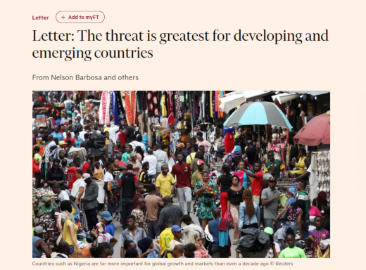
DECs are now confronted with a sudden stop as global liquidity conditions tighten and investors flee from risk: exposure to DECs remains a high-risk/high-return strategy, to be liquidated in times of crisis. In consequence, DECs face severe macroeconomic adjustment at precisely the moment when all available tools should be used to counter the public health crisis presented by COVID-19: some countries may be forced to tighten monetary policy in an attempt to retain access to the US dollar, while fiscal action may be constrained by fear of losing access to global markets. Foreign exchange reserves are unlikely to provide a sufficient buffer in all countries. This would have profound consequences for the global economy: DECs, both in the G20 and beyond, are now far more important for global growth and markets than even a decade ago. The failure of a large sovereign or quasi-sovereign borrower could trigger significant contagion.

There is an urgent need for action to prevent this crisis reaching catastrophic proportions in DECs. Despite long-standing calls for action, there is still no international lender of last resort. The only instruments currently available are IMF lending and foreign exchange (FX) swap lines between central banks. IMF loans typically impose fiscal tightening, which would be disastrous under current conditions. The US Federal Reserve stands ready to provide US dollars to a handful of major central banks: among DECs, only Mexico can access Fed and US Treasury swap lines under NAFTA provisions, and South Korea and Brazil have just had their arrangements re-opened. But these ad-hoc arrangements exclude a large proportion of DECs’ need for dollar liquidity.

We call for decisive action to constrain the financial flows currently transmitting the crisis to EMs. Capital controls should be introduced to curtail the surge in outflows, to reduce illiquidity driven by sell-offs in DECs’ markets, and to arrest declines in currency and asset prices. Implementation should be coordinated by the IMF to avoid stigma and prevent contagion. FX swap lines should be extended to include more DECs, in order to ensure access to US dollars. Finally, we concur with recent calls for greater provision of liquidity by the IMF using special drawing rights (SDRs) but this must take place without the imposition of pro-cyclical fiscal adjustment.

The unfolding crisis is one of the most serious in economic history. We must ensure that governments can do everything possible to protect their citizens. In our globally integrated economy, coordinated action is needed to minimise the externally-imposed constraints on developing and emerging countries as they face the triple threat of pandemic, recession and financial crisis.

Organising Signatories

Nelson Barbosa, Sao Paolo School of Economics

Richard Kozul-Wright, UNCTAD

Kevin Gallagher, Boston University

Jayati Ghosh, Jawaharlal Nehru University

Stephany Griffith-Jones, Columbia University

Adam Tooze, Columbia University

Bruno Bonizzi, University of Hertfordshire

Daniela Gabor, UWE Bristol

Annina Kaltenbrunner, University of Leeds

Jo Michell, UWE Bristol

Jeff Powell, University of Greenwich

Signatories

Adam Aboobaker, University of Massachusetts Amherst

Kuat Akizhanov, University of Birmingham and University of Bath

Siobhán Airey, University College Dublin

Ilias Alami, Maastricht University

Alejandro Alvarez, UNAM, México

Donatella Alessandrini, University of Kent

Jeffrey Althouse, University of Sorbonne Paris Nord

Carolina Alves, Girton College – University of Cambridge

Paul Anand, Open University and CPNSS London School of Economics

Phil Armstrong, University of Southampton Solent and York College

Paul Auerbach, Kingston University

Basani Baloyi, South Africa 

Frauke Banse, University of Kassel, Germany

Benoît Barthelmess, Le Club Européen

Pritish Behuria, University of Manchester

Kinnari Bhatt, Erasmus University Rotterdam

Samuele Bibi, Goldsmiths University

Joerg Bibow, Skidmore College

Pablo Bortz, National University of San Martín

Alberto Botta, University of Greenwich

Benjamin Braun, Institute for Advanced Study, Princeton

Louison Cahen-Fourot, Vienna University of Economics and Business

Jimena Castillo, University of Leeds, UK

Eugenio Caverzasi, Università degli Studi dell’Insubria

Jennifer Churchill, Kingston University, London

M Kerem Coban, GLODEM, Koc University, Turkey

Andrea Coveri, University of Urbino, Italy

Moritz Cruz, UNAM, Mexico

Florence Dafe, HfP/TUM School of Governance, Munich

Yannis Dafermos, SOAS University of London

Daria Davitti, Lund University, Sweden

Adam Dixon, Maastricht University

Cédric Durand, Université Sorbonne Paris Nord

Chandni Dwarkasing, University of Siena, Italy

Gary Dymski, University of Leeds

Ilhan Dögüs, University of Rostock, Germany

Carlo D’Ippoliti, Sapienza University of Rome

Dirk Ehnts, Technical University of Chemnitz

Luis Eslava, Kent Law School, University of Kent

Trevor Evans, Berlin School of Economics and Law

Andreas Exner, University of Graz

Karina Patricio Ferreira Lima, Durham University

José Bruno Fevereiro, The Open University Business School

Andrew M. Fischer, Erasmus University Rotterdam

Giorgos Galanis, Goldsmiths, University of London

Santiago José Gahn, Università degli studi Roma Tre

Jorge Garcia-Arias, University of Leon, Spain and SOAS, University of London

Alicia Girón – UNAM-MEXICO

Thomas Goda, Universidad EAFIT, Colombia

Antoine Godin, University Sorbonne Paris Nord

Gabriel Gómez, UNAM, México

Jesse Griffiths, Overseas Development Institute

Diego Guevara, National University of Colombia

Alexander Guschanski, University of Greenwich

Sarah Hall, University of Nottingham

James Harrison, Prof, University of Warwick

Nicolas Hernan Zeolla, National University of San Martin, Argentina

Hansjörg Herr, Berlin School of Economics and Law

Elena Hofferberth, University of Leeds

Jens Holscher, Bournemouth University

Peter Howard-Jones, Bournemouth University

Bruno Höfig, SOAS, University of London

Roberto Iacono, Norwegian University of Science and Technology

Stefanos Ioannou, University of Oxford

Andrew Jackson, University of of Surrey 

Juvaria Jafri, City University of London

Frederico G. Jayme, Jr, Federal University of Minas Gerais, Brazil

Emily Jones, University of Oxford

Ewa Karwowski, University of Hertfordshire

Y.K. Kim, University of Massachusetts Boston

Stephen Kinsella, University of Limerick

Kai Koddenbrock, University of Frankfurt

George Krimpas, University of Athens

Sophia Kuehnlenz, Manchester Metropolitan University

Ingrid Harvold Kvangraven, University of York

Annamaria La Chimia, University of Nottingham

Dany Lang, Université Sorbonne Paris Nord

Jean Langlois, Le Club Européen

Christina Laskaridis, SOAS, University of London

Lyla Latif, University of Nairobi

Thibault Laurentjoye, École des Hautes Études en Sciences Sociales (EHESS), Paris

Dominik A. Leusder, London School of Economics

Noemi Levy-Orlik, UNAM, Mexico

Gilberto Libanio, Federal University of Minas Gerais, Brazil

Duncan Lindo, Vrije Universiteit Brussel

Lorena Lombardozzi, Open University

Anne Löscher, University of Siegen, Germany; University of Leeds

Birgit Mahnkopf, Prof.i.R., Berlin School of Economy and Law

Pedro Mendes Loureiro, University of Cambridge

Victor Isidro Luna, UNAM

Jonathan Marie, Université Sorbonne Paris Nord

Norberto Montani Martins, Federal University of Rio de Janeiro, Brazil

Olivia Bullio Mattos, St. Francis College, New York, USA

Andrew Mearman, University of Leeds

Monika Meireles, UNAM

Thorvald Grung Moe, Levy Economics Institute

Lumkile Mondi, University of the Witwatersrand, South Africa

Thanti Mthanti, University of the Witwatersrand, South Africa

Susan Newman, Open University

Howard Nicholas, International Institute of Social Studies, Erasmus University Rotterdam

Maria Nikolaidi, University of Greenwich

Patricia Northover, University of the West Indies, Jamaica

Cem Oyvat, University of Greenwich

Oktay Özden, Marmara University, Turkey

Vishnu Padayachee, University of the Witwatersrand 

Rafael Palazzi, PUC-Rio, Brazil

José Gabriel Palma, Cambridge University and USACH

Marco Veronese Passarella, University of Leeds

Jonathan Perraton, University of Sheffield

Nicolás M. Perrone, Universidad Andres Bello, Viña del Mar

Keston K. Perry, UWE Bristol

Mate Pesti, UWE Bristol

Karl Petrick, Western New England University

Christos Pierros, University of Athens

Leonhard Plank, TU Wien

Jose Pérez-Montiel, University of the Balearic Islands, Spain

Hao Qi, Renmin University of China

Mzukisi Qobo, Wits Business School, University of Witwarsrand

Joel Rabinovich, University of Leeds

Dubravko Radosevic, University of Zagreb

Miriam Rehm, University of Duisburg-Essen

Marco Flávio da Cunha Resende, Federal University of Minas Gerais, Brazil

Lena Rethel, University of Warwick

Sergio Rossi, C University of Fribourg, Switzerland

Maria Jose Romero, Eurodad

Roy Rotheim, Skidmore College

Josh Ryan-Collins, UCL Institute for Innovation and Public Purpose

Alfredo Saad Filho, King’s College London

Lino Sau, University of Torino, Italy

Malcolm Sawyer. Emeritus Professor of Economics, University of Leeds

Anil Shah, University of Kassel

Dawa Sherpa, Jawaharlal Nehru University 

Hee-Young Shin, Wright State University

Farwa Sial, Global Development Institute, University of Manchester

Crystal Simeoni, FEMNET, Nairobi, Kenya

Engelbert Stockhammer, King’s College London

Ndongo Samba Sylla, Dakar

Carolyn Sissoko, UWE Bristol

Celine Tan, University of Warwick

Gyekye Tanoh, Accra

Daniela Tavasci, School of Economics and Finance, Queen Mary University of London

Andrea Terzi, Franklin University Switzerland 

Daniele Tori, Open University Business School

Gamze Erdem Türkelli, University of Antwerp

Esra Ugurlu, University of Massachusetts Amherst

Ezgi Unsal, Kadir Has University

Tara Van Ho, University of Essex 

Sophie Van Huellen, SOAS University of London

Frank Van Lerven, New Economics Foundation

Elisa Van Waeyenberge, SOAS University of London

Paolo Vargiu, University of Leicester

Luigi Ventimiglia, School of Economics and Finance, Queen Mary University of London

Apostolos Vetsikas, University of Thessaly, Greece

Davide Villani, The Open University and Goldsmiths, University of London

Camila Villard Duran, University of Sao Paulo

Pablo Wahren, University of Buenos Aires

Neil Warner, London School of Economics

Mary Wrenn, UWE Bristol

Joscha Wullweber, University of Witten/Herdecke

Devrim Yilmaz, Université Sorbonne Paris Nord

MMT: History, theory and politics

Originally published in Spanish as “¿De dónde viene el dinero?” by Política Exterior

Modern monetary theory, or MMT as it is widely known, has achieved remarkable visibility in recent years. Despite the title, MMT can resemble a political campaign as much as a monetary theory, characterised by activists promoting job guarantee schemes alongside more scholarly activity. The core ideas of MMT coalesced in the early 1990s, developed and promoted by a small group who largely bypassed academia, instead using blogs to accumulate a dedicated band of followers. As Bill Mitchell, one of the founders of MMT, said at the recent “International MMT Conference” in New York, “This is the first body of economic theory that has grown through activists”. In recent years that following has expanded substantially, leading to global prominence for key MMT figures, and widespread media coverage and commentary.

The main propositions of MMT are derived from one simple observation: a country with its own currency cannot run out of that currency. The U.S. government cannot run out of dollars because dollars are issued by the Federal Reserve, which is controlled by the U.S government. As a result, the U.S. government will never face a situation in which it cannot find the money to pay the interest on its debt, to hire workers, or to purchase goods and services. This, MMT proponents argue, turns conventional thinking on its head: mainstream economics promotes misconceptions about public debt, imposing false barriers to public spending. In contrast, it is claimed, MMT identifies the true constraints faced by currency-issuing governments, liberating policy-makers from misguided concerns about “finding the money” to pay for government spending.

The reality, as we shall see, is a bit more complicated. But first, some history. The MMT story starts with Warren Mosler, an ex-Wall Street trader who, in the 1980s, founded both a hedge fund and a supercar manufacturer, before relocating to the Virgin Islands, a Caribbean tax haven. In the early 1990s, Mosler took his ideas on sovereign debt to Donald Rumsfeld who sent him to Arthur Laffer (of “Laffer Curve” fame). Laffer told Mosler that the high priests of economic orthodoxy were unlikely to be interested in his ideas, and suggested he instead try the Post-Keynesians: a group of left-leaning non-mainstream economists. Mosler joined a Post-Keynesian email discussion list and found common ground with academics such as L. Randall Wray and his colleagues in the US, and Bill Mitchell in Australia. The group embarked on the project of developing a new synthesis of ideas on monetary economics.

Mosler convinced the group that the commonly held view that taxes provide the funds required for government spending is false. Instead, when a currency-issuing government spends, it creates new money: when the U.S. government makes a payment, new dollars are brought into existence at the point of expenditure. Discussions framed in terms such as “where will the government find the money?” are therefore based on a flawed understanding of the monetary system, Mosler argues.

According to Mosler, the purpose of taxation is instead to create the demand for government-issued currency. In the absence of taxes, Mosler contends, there would be no demand for essentially worthless pieces of paper. But in declaring and imposing the unit (the dollar) in which tax obligations must be discharged, the government ensures widespread use and acceptability of its currency.

These ideas turned out to be compatible with those of Randall Wray, an academic who was working on “Chartalist” ideas concerning the role of the state in defining and enforcing what is used as money. In the Chartalist view, money is not and has never been a commodity such as gold. Instead, money is essentially a system of IOUs that keeps track of credit and debit positions across a society too large and complex to rely on direct credit relationships. While credit theories of money have a longstanding tradition, the novelty of Chartalism lies with the claim that “money is a creature of the state”. By imposing the use of its own currency, Chartalists argue, the government, as monopoly issuer of that currency, attains powers not available to any other economic actor.

The core of MMT is a synthesis of Mosler and Wray’s ideas about government money with elements such as Abba Lerner’s “functional finance”. Lerner argues that government finances are not appropriate targets for government policy. Instead, the government should judge its actions on the basis of real outcomes, such as the level of employment. When combined with Mosler’s assertion that a currency-issuing government is never unable to service its debt, the claim that the appropriate target for macroeconomic policy is full employment appears logical. For MMT, the limit to government spending is therefore not financial but real, imposed by the physical capacity of the economic system to produce goods and services. The limit to fiscal activism is therefore the “inflation barrier” – the point at which increases in government spending generate rising prices, rather than higher employment and production.

The last piece of the MMT puzzle is the “employer of last resort” policy. Functional finance says that government spending should be used to eliminate unemployment – but there is a catch. As unemployment is reduced, inflation is likely to strengthen. It is unlikely that true zero unemployment can be achieved simply by raising government spending: at some point inflation will set in.

The employer of last resort (ELR) is MMT’s proposed solution to this problem. The policy is deceptively simple: the government should stand ready to employ all those who want work, offering a wage set at a level below the prevailing private sector wage rate. The justification claimed is twofold. First the policy will eliminate the social ill of unemployment: all those who want work will have it. Second, by setting wages below the level in the private sector, the ELR will create a “nominal anchor”: the below-market-rate ELR wage will restrain wage demands across the economy, preventing inflation, even in the absence of unemployment. When inflation sets in, the government should respond by reducing total spending, leading to lay-offs in the private sector. These laid off workers will be picked up by the ELR, at lower wages than the private sector. This increase in the “buffer stock” of ELR workers will serve to dampen wage demands in the private sector, reducing inflationary pressure.

These three elements: sovereign money, functional finance and the employer of last resort comprise the theoretical and policy core of MMT.

Before assessing whether this provides a sound basis for policy, we need to first briefly consider some history of the relationship between economic theory and macroeconomic policy. In the advanced economic nations, the post-war years were characterised by rapid growth and very low unemployment rates. By the middle of 1970s, this benign macroeconomic environment had given way to oil price hikes, the breakdown of the Bretton Woods managed exchange rate system and rising labour militancy. Policy-makers switched their focus from employment to inflation: the influence of Milton Friedman’s monetarism led to a growing belief that using macroeconomic policy for anything other than controlling inflation was futile, and that employment should be abandoned as a policy target. Through the 1980s and 1990s, academic economics coalesced around an increasingly mathematical formalisation of Friedman’s ideas (confusingly, this acquired the title of “New Keynesian economics”). While mathematically complex, this boils down to three main propositions.

First, total spending by households and businesses – what economists refer to as aggregate demand – is determined, in the short run, by the rate of interest. Since the rate of interest is assumed to be under the control of the central bank, total spending is therefore under direct policy control. Second, inflation is determined by two factors: firstly by total spending relative to the productive capacity of the economy and, secondly, by expectations about future inflation. In this view, if inflation is too high, the central bank should raise the rate of interest, reducing total spending and thus reducing inflationary pressure. The speed at which inflation will return to target will depend on the “credibility” of the central bank: if households and businesses believe that the central bank is serious about getting inflation under control, even at the cost of higher short-run unemployment, then inflation will adjust quickly. The conclusion – the third proposition – is that the optimal way to implement macroeconomic policy is for an independent central bank to adopt a policy rule, explicitly stating how it will adjust interest rates when inflation is above target. This, it is argued, is the most effective way to ensure that the central bank is credible – and is not susceptible to politicians seeking to temporarily lower unemployment as a way to improve their electoral prospects.

A small group of dissenting “heterodox” economists maintained a position of opposition to the ascendancy of monetarist ideas, arguing that Friedman’s diagnosis relied on an over-simplified view of inflation as the result of “too much money chasing too few goods”. Drawing inspiration from Keynes and his contemporaries Michal Kalecki, Joan Robinson and Nicholas Kaldor, this group adopted the term “Post-Keynesian” to distinguish their position from that of the mainstream. The Post-Keynesians rejected the key monetarist assertion that the central bank can always influence economic activity by adjusting either the quantity of money or the policy rate of interest. As Keynes put it, monetary policy is like “pushing on a string”: tighter policy will dampen economic activity, but looser policy will not automatically act as a stimulus. Fiscal policy is therefore required for macroeconomic stabilisation.

From around the mid-1970s, Post-Keynesian economics was characterised by a transatlantic division of labour. In the UK, with Cambridge at the centre, much attention was focused on growth and distribution. In the US, a closer interest was taken in monetary and financial issues. It was with members of this group of US Post-Keynesians that Mosler formed an alliance in the 1990s. Mosler’s financial backing enabled institutional support at the University of Missouri-Kansas, where several prominent MMT developers gained employment, including a PhD training programme to incubate the next generation of MMT advocates.

While the theoretical core of MMT is close to the ideas of Post-Keynesian economics, MMT stole a march on their Post-Keynesians colleagues in exploiting social media and non-academic activism. With hindsight, however, these tactics turn out to be something of a double-edged sword: success relied on the use of slogans such as “money doesn’t grow on rich people”, “taxes don’t pay for spending” and “money is no object”. These slogans, and the zeal with which advocates adopted them, arguably serve to obscure the underlying ideas, making MMT claims appear more groundbreaking than is really the case.

Take the claim that “taxes don’t pay for spending”. It has long been taught in elementary macroeconomics classes that government spending adds to total national expenditure, while taxes are a deduction. The two variables are treated as moving independently of one another: taxation doesn’t constrain government spending. Since at least the time of Keynes, it has been understood that tax plays an important macroeconomic role in limiting total private sector spending, thus ensuring that economic capacity is available for government programmes. Whether this function should be characterised as taxes “paying for” spending is perhaps semantic.

Textbooks usually explain that the gap between government spending and taxation is covered by issuance of government bonds. MMT goes further, claiming that government spending is not financed by either taxes or bond issuance: Governments first spend, creating new money, then withdraw money from circulation by imposing taxes or issuing bonds. As a result, MMT proponents claim, taxes can be cut dramatically, without affecting the ability of government to spend, while bond issuance can be eliminated entirely.

Does MMT provide a good guide for policy? MMT proponents tend to deny that MMT provides policy proposals. Instead, it is claimed, MMT is a “lens” through which one comprehends the true nature of the monetary system. MMT is not a policy package, it is argued, because MMT is simply a description of how the system already works.

This claim stretches credibility. Putting the ELR proposal aside, MMT proponents do make policy proposals (such as those already noted). The common feature of such proposals is the use of deficit monetisation: issuing central bank money directly to pay for government programmes. For example, Warren Mosler proposes abolishing all payroll taxes, while Stephanie Kelton has argued that the Green New Deal, a massive public spending programme championed by the left of Democratic Party, can be implemented without needing to tax the wealthy.

Complaints by proponents that MMT is mischaracterised as “printing money” are therefore misplaced. The suggestion that MMT claims “deficits don’t matter” likewise causes protest: MMT proponents respond that deficits matter, but what matters is the so-called “real resource constraint”. As a result, as MMT proponents correctly note, deficits can be too small as well as too large – an obvious current example is Germany, where demand clearly falls short of real constraints, and there is substantial capacity for fiscal expansion. Despits this, MMT complaints are again misleading: MMT does argue that there is no financial constraint to government deficits. While it is almost certainly the case that the US and other advanced nations still have substantial fiscal space, despite running large deficits in some cases, the MMT claim is too extreme; at some point, fiscal limits will be reached even in rich nations. For countries further down the international currency hierarchy which face binding externally-imposed constraints related to foreign exchange needs, fiscal limits are very real.

Further, despite MMT proponents emphasising the “inflation barrier” as the true limit to deficit spending, little effort is devoted to the crucial questions of how real resources are to be mobilised: how to ensure that large government spending programmes such as the Green New Deal can be implemented without hitting supply side bottlenecks, capacity limits and political resistance. In framing everything in monetary terms, rather than real economic activity, MMT therefore obscures rather than illuminates important macroeconomic relationships.

Once the esoteric use of language and the more extreme claims are stripped away, there is arguably a rather conventional core to MMT. US economists JW Mason and Arun Jayadev argue that, in policy terms, MMT effectively amounts to a reversal of the “consensus assignment”. This refers to the idea that the two main tools of macroeconomic management, fiscal policy and monetary policy, should each be assigned a single target. The consensus assignment is that monetary policy (setting interest rates and, more recently, quantitative easing) should be used to manage aggregate demand, while fiscal policy is used to maintain sustainable debt-to-GDP ratios. In contrast, MMT proposes the use of fiscal policy to manage demand, and monetary policy (in the form of deficit monetisation and zero interest rates) to manage the public finances.

MMT is usually portrayed as a left-wing economic programme: Stephanie Kelton is an economic advisor to Bernie Sanders and Alexandria Ocasio-Cortez has said that MMT should be “part of the conversation”. But although much of the MMT activist base is on the left, the relationship between MMT and politics is more complex. The line that “money doesn’t grow on rich people” can potentially play well on the right, as much as the left. As already noted, Mosler, a self-described “Tea Party Democrat” proposes the abolition of payroll taxes. Bill Mitchell argues that MMT is politically neutral, and MMT insights can inform either left- or right-wing political programmes. Care therefore needs to be taken when associating government deficits with the political left: US Republicans use deficit scaremongering to constrain public spending by Democrat administrations, but Republican governments are often less fiscally cautious in office — Trump’s tax cuts provide a recent example. Similarly, in the UK, after nearly a decade of government cuts premised on the false threat of a run on bond markets, the Conservative government has decided to embrace deficits, cutting taxes and making eye-catching spending claims.

The ideas of MMT could also be adopted by political groups that combine socially right-wing ideas with activist fiscal policy. In their recent book, “Reclaiming The State”, Bill Mitchell and his co-author Thomas Fazi note the successful use of deficit monetisation in Nazi Germany, while decrying the “tragedy” of the Left’s focus in recent decades on “identity politics”: opposition to racism, homophobia and other forms of bigotry. This, Mitchell argues, serves to radicalise the “ethnocentrism of the proletariat”. This framing of MMT in terms of national sovereignty will have obvious appeal to those wishing to implement nativist policies, such as restricting migration, while using deficit spending to ensure employment for those on the inside.

MMT has had remarkable success in opposing needless deficit hysteria and in popularising more enlightened ideas on macroeconomic management than those prevailing since the rise of monetarism in the 1970s. Recent events have demonstrated the ineffectiveness of monetary policy as a demand management tool: it is now widely accepted that fiscal policy must play a more active role. MMT activists should therefore be commended: they have succeeded where other heterodox economists have failed in popularising these important ideas. But the use of obscurantist language, oversimplification of complex issues and the tendency to make excessive claims ultimately undermines their case.

Time will tell if MMT is destined to become a passing phase or a more permanent “part of the conversation”. What seems more certain is that the days of reliance on monetary policy as the sole macroeconomic stabilisation tool are over: fiscal policy is back on the agenda.

Kelton and Krugman on IS-LM and MMT

The MMT debates continue apace. New critiques — the good, the bad and the ugly — appear daily. Amidst the chaos, a guest post on Alphaville from three MMT authors stood out: the piece responded directly to various criticisms while discussing the policy challenges associated with controlling demand and inflation when fiscal policy is the primary macro stabilisation tool. These are the debates we should be having.

Unfortunately, it is one step forward, two steps backwards: elsewhere Stephanie Kelton and Paul Krugman have been debating across the pages of the Bloomberg and the New York Times websites. The debate is, to put it politely, a mess.

Krugman opened proceedings with a critique of Abba Lerner’s Functional Finance: the doctrine that fiscal policy should be judged by its macroeconomic outcomes, not on whether the financing is “sound”. Lerner argued that fiscal policy should be set at a position consistent with full employment, while interest rates should be set at a rate that ensures “the most desirable level of investment”. Krugman correctly notes the lack of  precision in Lerner’s statement on interest rates. He then argues that, “Lerner neglected the tradeoff between monetary and fiscal policy”, and that if the rate of interest on government debt exceeds the rate of growth, either the debt to GDP ratio spirals out of control or the government is forced to tighten fiscal policy.

Kelton hit back, arguing that Krugman’s concerns are misplaced because interest rates are a policy variable: the central bank can set them at whatever level it likes. Kelton points out that Krugman is assuming a “crowding out” effect: higher deficits lead to higher interest rates. Kelton argues that instead of “crowding out”, Lerner was concerned about “crowding in”: the “danger” that government deficits would push down the rate of interest, stimulating too much investment. Putting aside whether this is an accurate description of Lerner’s view, MMT does diverge from Lerner on this issue: since MMT rejects a clear link between interest rates and investment,  the MMT proposal is simply to set interest rates at a low level, or even zero, and leave them there.

So far, this looks like a straightforward disagreement about the relationship between government deficits and interest rates: Krugman says deficits cause higher interest rates, Kelton says they cause lower interest rates (although she also says interest rates are a policy variable — this apparent tension in Kelton’s position is resolved later on)

Krugman responded. This is where the debate starts to get messy. Krugman takes issue with the claim that the deficit should be set at the level consistent with full employment. He argues that at different rates of interest there will be different levels of private sector spending, implying that the fiscal position consistent with full employment varies with the rate of interest. As a result, the rate of interest isn’t a pure policy variable: there is a tradeoff between monetary and fiscal policy: with a larger deficit, interest rates must be higher, “crowding out” private investment spending.

Krugman’s argument involves two assumptions: 1) there exists a direct causal relationship between the rate of interest and the level of private investment expenditure, and, 2) the central bank will react to employment above “full employment” with higher interest rates. He illustrates this using an IS curve and a vertical “full employment” line (see below). He declares that “this all seems clear to me, and hard to argue with”.

250219krugman1-jumbo

At this point the debate still appears to remain focused on the core question: do government deficits raise or lower the rate of interest? By now, Krugman is baffled with Kelton’s responses:

It seems as if she’s saying that deficits necessarily lead to an increase in the monetary base, that expansionary fiscal policy is automatically expansionary monetary policy. But that is so obviously untrue – think of the loose fiscal/tight money combination in the 1980s – that I hope she means something different. Yet I can’t figure out what that different thing might be.

This highlights two issues: first, how little of MMT Krugman has bothered to absorb, and, second, how little MMTers appear to care about engaging others in a clear debate. Kelton, following the MMT line, is tacitly assuming that all deficits are monetised and that issuing bonds is an additional, and possibly unnecessary, “sterilisation” operation. Under these assumptions, deficits will automatically lead to an increase in central bank reserves and therefore to a fall in the money market rate of interest. But Kelton at no point makes these assumptions explicit. To most people, a government deficit implicitly means bond issuance, in correspondence with the historical facts.

So Krugman and Kelton have two differences in assumptions that matter here. First, Krugman assumes a mechanical relationship between interest rates and investment and thus a downward sloping IS curve, while Kelton rejects this relationship. Second, they are assuming different central bank behaviour. Krugman assumes that the central bank will react to fiscal expansion with tighter monetary policy in the form of higher interest rates: the central bank won’t allow employment to exceed the “full employment” level. Kelton assumes, firstly, that fiscal policy can be set at the “full employment” level, without any direct implications for interest rates and, secondly, that deficits are monetised so that money market rates fall as the deficit expands.

The “debate” heads downhill from here. Krugman asks several direct questions, including “[does] expansionary fiscal policy actually reduce interest rates?”. Kelton responds, “Answer: Yes. Pumping money into the economy increases bank reserves and reduces banks’ bids for federal funds. Any banker will tell you this.” Even now,  neither party seems to have identified the difference in assumptions about central bank behaviour.

The debate then shifts to IS-LM. Krugman asks if Kelton accepts the overall framework of discussion — the one he previously noted “all seems clear to me, and hard to argue with”. Kelton responds that, no, MMT rejects IS-LM because it is “not stock-flow consistent”, while also correctly noting that Krugman simply assumes that investment is a mechanical function of the rate of interest.

In fact, Krugman isn’t even using an IS-LM model — he has no LM curve — so the “not stock flow consistent” response is off target. The stock-flow issue in IS-LM derives from the fact that the model solves for an equilibrium between equations for the stock of money (LM), and investment and saving (IS) which are flow variables. But without the LM curve it is a pure flow model: Krugman is assuming, as does Kelton, that the central bank sets the rate of interest directly. So Kelton’s claim that “his model assumes a fixed money supply, which paves the way for the crowding-out effect!” is incorrect.

Similarly, Kelton’s earlier statement that Krugman “subscribes to the idea that monetary policy should target an invisible ‘neutral rate'” makes little sense in the context of Krugman’s IS model: there is no “invisible” r* in a simple IS model of the type Krugman is using: the full employment rate of interest can be read straight off the diagram for any given fiscal position.

Krugman then took to Twitter, calling Kelton’s response “a mess”, while still apparently failing to spot that they are talking at cross purposes. Kelton hit back again arguing that,

The crude, IS-LM interpretation of Keynes demonstrates that, under normal conditions, an increase in deficit spending will push up interest rates and lead to some crowding-out of investment spending. There is no room for a technical analysis of monetary operations in that framework.

Can this discussion be rescued? Can MMT and IS-LM be reconciled? The answer, I think, turns out to be, “yes, sort of”.

I wasn’t the only person pondering this question: several people on Twitter went back to this post by Nick Rowe where he tries to “reverse engineer” MMT using the IS-LM model, and comes up with the following diagram:

Rowe-IS-LM
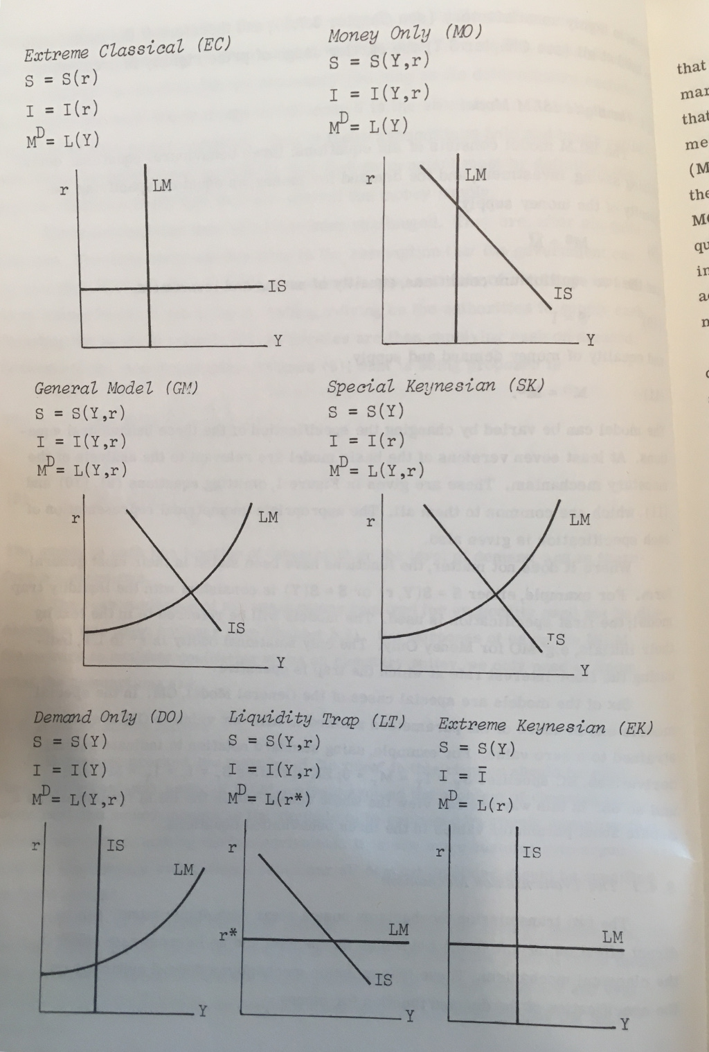
Does this help? I think it does. In fact, this is exactly the diagram used by Victoria Chick in 1973, in The Theory of Monetary Policy, to describe what she calls the “extreme Keynesian model” (bottom right):

Chick-Theory-Monetary-Policy-scaled

So how do we use this diagram to resolve the Krugman-Kelton debate? Before answering, it should be noted that MMTers are correct to point out problems with the IS-LM framework. Some are listed in this article by Mario Seccareccia and Marc Lavoie who conclude that IS-LM should be rejected, but “if one were to hold one’s nose,” the “least worst” configuration is what Chick calls the “extreme Keynesian” version.

To see how we resolve the debate, and at the risk of repeating myself, recall that Krugman and Kelton are talking about two different central bank reactions. In Krugman’s IS model, the central bank reacts to looser fiscal policy with higher interest rates. Kelton, on the other hand, is talking about how deficit monetisation lowers the overnight money market rate. Kelton’s claim that a government deficit reduces “interest rates” is largely meaningless: it is just a truism. Flooding the overnight markets with liquidity will quickly push the rate of interest to zero, or whatever rate of interest the central bank pays on reserve balances. It is a central bank policy choice: the opposite of the one assumed by Krugman.

But what effect will this have on the interest rates which really matter for investment and debt sustainability: the rates on corporate and government debt? The answer is “it depends” — there are far too many factors involved to posit a direct mechanical relationship.

This brings a problem that is lurking in the background into sight. Both Kelton and Krugman are talking about “interest rates” or “the interest rate” as if there were a single rate of interest, or that all rates move together — the yield curve shifts bodily with movements of the policy rate. As the chart below shows, even for government debt alone this is a problematic assumption.

yc

Now, in the original IS-LM model, the LM curve is supposed to show how changes in the government controlled “money supply” affects the long term bond rate of interest. This is because, for Keynes, the rate of interest is the price of liquidity: by giving up liquidity (money) in favour of bonds, investors are rewarded with interest payments. But the problem with this is that we know that central banks don’t set the “money supply”: they set a rate of interest. So, it has become customary to draw a horizontal MP curve, allegedly representing an elastic supply of money at the rate of interest set by the central bank. But note that in switching from a sloping to a horizontal LM curve, the “interest rate” has switched from the long bond rate to the rate set by the central bank.

So how is the long bond rate determined in the horizontal MP model? The answer is it isn’t. As in the more contemporary three-equation IS-AS-MP formulation, it is just assumed that the central bank fixes the rate of interest that determines total spending. In switching from the upward sloping LM curve to a horizontal MP curve, the crude approximation to the yield curve in the older model is eliminated.

What of the IS curve? Kelton is right that a mechanical relationship between interest rates and investment (and saving) behaviour is highly dubious. If we assume that demand is completely interest-inelastic, then we arrive at the “extreme Keynesian” vertical IS curve. But does Kelton really think that sharp Fed rate hikes will have no effect on total spending? I doubt it. As Seccareccia and Lavoie note, once the effects of interest rates on the housing market are included, a sloping-but-steep IS curve seems plausible.

Now, does the “extreme Keynesian” IS-LM model, all the heroic assumptions notwithstanding, represent the MMT assumptions? I think, very crudely, it does. The government can set fiscal policy wherever it likes, both irrespective of interest rates and without affecting interest rates: the IS curve can be placed anywhere along the horizontal axis. Likewise, the central bank can set interest rates to anything it likes, again without having any effect on total expenditure. This seems a reasonable, if highly simplified approximation to the standard MMT assumptions that fiscal policy and monetary policy can be set entirely independently of each other.

But is it useful? Not really, other than perhaps in showing the limitations of IS-LM. The only real takeaway is that we deserve a better quality of economic debate. People with the visibility and status of Kelton and Krugman should be able to identify the assumptions driving their opponent’s conclusions and hold a meaningful debate about whether these assumptions hold — without requiring some blogger to pick up the pieces.

Misunderstanding MMT

MMT continues to generate debate. Recent contributions include Jonathan Portes’ critique in Prospect and Stephanie Kelton’s Bloomberg op-ed downplaying the AOC and Warren tax proposals.

Something that caught my eye in Jonathans’ discussion was this quote from Richard Murphy: “A government with a balanced budget necessarily denies an economy the funds it needs to function.” This is an odd claim, and not something that follows from MMT.

Richard has responded to Jonathan’s article, predictably enough with straw man accusations, and declaring, somewhat grandiosely, that “the left and Labour really do need to adopt the core ideas of modern monetary theory … This debate is now at the heart of what it is to be on the left”

Richard included a six-point definition of what he regards to be the core propositions of MMT. Paraphrasing in some cases, these are:

  1. All money is created by the state or other banks acting under state licence
  2. Money only has value because the government promises to back it …
  3. … because taxes must be paid in government-issued money
  4. Therefore government spending comes before taxation
  5. Government deficits are necessary and good because without them the means to make settlement would not exist in our economy
  6. This liberates us to think entirely afresh about fiscal policy

Of these, I’d say the first is true, with some caveats, the second and third are partially true, and the fourth is sort of true but also not particularly interesting. I’ll leave further elaboration for another time, because I want to focus on point five, which is almost a restatement of the quote in Jonathan’s Prospect piece.

This claim is neither correct nor part of MMT. I don’t believe that any of the core MMT scholars would argue that deficits are required to ensure that there is sufficient money in circulation. (Since Richard uses the term “funds” in the first quote and “means [of] settlement” in the second, I’m going to assume he means money).

To see why, consider what makes up “money” in a modern monetary system. Bank deposits are the bulk of the money we use. These are issued by private banks when they make loans. Bank notes, issued by the Bank of England make up a much smaller proportion of the money in the hands of the public. Finally, there are the balances that private banks hold at the Bank of England, called reserves.

What is the relationship between these types of money and the government surplus or deficit? The figure below shows how both deposits and reserves have changed over time, alongside the deficit.

uk-money-supply-deficit

Can you spot a connection between the deficit and either of the two money measures? No, that’s because there isn’t one — and there is no reason to expect one.

Reserves increase when the Bank of England lends to commercial banks or purchases assets from the private sector. Deposits increase when commercial banks lend to households or firms. Until 2008, the Bank of England’s inflation targeting framework meant it aimed to keep the amount of reserves in the system low — it ran a tight balance sheet. Following the crisis, QE was introduced and the Bank rapidly increased reserves by purchasing government debt from private financial institutions. Over this period, and despite the increase in reserves, the ratio of deposits to GDP remained pretty stable.

The quantity of neither reserves nor deposits have any direct relationship with the government deficit. This is because the deficit is financed using bonds. For every £1bn of reserves and deposits created when the government spends in excess of taxation, £1bn of reserves and deposits are withdrawn when the Treasury sells bonds to finance that deficit.

This is exactly what MMT says will happen (although MMT also argues that these bond sales may not always be necessary). So MMT nowhere makes the claim that deficits are required to ensure that the system has enough money to function.

It is true that the smooth operation of the banking and financial system relies on well-functioning markets in government bonds. During the Clinton Presidency there were concerns that budget surpluses might lead the government to pay back all debt, thus leaving the financial system high and dry.

But the UK is not in any danger of running out of government debt. Government surpluses or deficits thus have no bearing on the ability of the monetary system to function.

The macroeconomic reason for running a deficit is straightforward and has nothing to do with money. The government should run a deficit when the desired saving of the private sector exceeds the sum of private investment expenditure and the surplus with the rest of the world. This is not an insight of MMT: it was stated by Kalecki and Keynes in the 1930s.

If a debate about MMT really is at “the heart of what it is to be on the left” then Richard might want to take a break to get up to speed on MMT (and monetary economics) before that debate continues.

Argentina: From the “confidence fairy” to the (still devilish) IMF

Guest post by Pablo Bortz and Nicolás Zeolla, Researchers at the Centre of Studies on Economics and Development, IDAES, National University of San Martín, and CONICET, Argentina.

In recent days, it has become customary to recall the issuance of a USD 2.75 billion 100-year bond in June 2017. This was the most colourful event of the short-lived integration of Argentina into international capital markets, beginning in December 2015. Last week, Argentina returned to the front pages of the financial press when the government requested financial assistance to the IMF amidst capital flight and a run against the peso that authorities were struggling to stop.

This is the most recent episode in the typical cycle of an emerging economy entering financial markets, suffering a balance of payments crisis and adopting an IMF-sponsored stabilization program. It starts with the claim that we are now a respected member of the international community, with presence in the Davos forum, and the promise that this time, finally, the international “confidence fairy” will awaken and investment will flood the country because of all the profit opportunities this forgotten economy has to offer. When the fairy proves to be an hallucination, we find ourselves at the steps of the IMF, facing demands, as always, for fiscal consolidation and structural reform.

When explaining this story, it is important to have some background on the Argentineans’ fascination with the dollar, and on some very recent political history. Because of its history of financial crises and its underdeveloped capital markets, there are very few savings instruments available to the non-sophisticated investor: real estate, term deposits, and dollars. Real estate prices are denominated in dollars, but you need a lot of dollars (relative to income) to buy a house. So buying dollars is pretty much a straightforward investment in uncertain times, i.e. most of the time.

Added to that, Argentina has a higher degree of exchange rate pass-through than other developing countries. The main exporters also dominate the domestic market for cooking oil and flour; oil and energy prices are dollarized; and exchange rate movements are very closely followed at times of wage bargaining. Unlike other emerging countries, and despite the sneering of some government officials, in a semi-dollarized (or bimonetary) economy such as Argentina exchange-rate pass-through is alive and kicking, which discourages large devaluations.

It is important to remember that the previous administration of Cristina Fernandez de Kirchner had implemented pervasive capital and exchange controls, which led to the development of a (relatively small) parallel market, with almost a 60% gap between the official and the parallel exchange rate. As soon as the Macri government took power in December 2015, it lifted all exchange rate controls. The official exchange rate (10 pesos per dollar) moved towards the parallel (16 pesos per dollar), and it is one of the reasons for the increase in the inflation rate, from 24% in 2015 to 41% by the end of 2016.

The new authorities also made two big moves. One was cancelling all the debt with vulture funds with new borrowing. This officially marked the return of Argentina to international capital markets. The second move, by the central bank (now lead by Federico Sturzenegger, an MIT graduate and disciple of Rudi Dornbusch), was the adoption of an inflation-targeting regime, with a mind-set that preferred freely floating exchange rates, and not much concern for current account deficits[1].

But looking at the external front, one may even be forgiven for asking: why did this crisis take so long to burst? Argentina was haemorrhaging dollars for many years, and with no sign of reversal: since 2016 the domestic non-financial sector acquired an accumulated amount of USD 41 billion in external assets. During the same period, the current account deficit totalled another USD 30 billion, in the form of trade deficit, tourism deficit, profit remittances by foreign companies and increasing interest payments.

The well-known factor that allowed all these trends to last until now is the foreign borrowing spree that involved the government, provinces, firms, and the central bank, including the inflow from short-term investors for carry trade operations. In the case of debt issuance, since 2016 the central government, provinces and private companies, have issued a whopping USD 88 billion of new foreign debt (13% of GDP).  In the case of carry trade operations, since 2016 the economy recorded USD 14 billon of short-term capital inflows (2% of GDP). The favourite peso-denominated asset for this operations were the debt liabilities of the central bank called LEBAC (Letters of the Central Bank).  Because of this, the outstanding stock of this instrument has now become the centre of all attention.

It is important to understand the LEBACs. They were originally conceived as an inter-bank and central bank liquidity management instrument. Since the lifting of foreign exchange and capital controls and the adoption of inflation targeting, the stock of LEBACs grew by USD 18 billion. Moreover, the composition of holders has changed significantly since 2015: At that time, domestic banks held 71% of the stock, and other investors held 29%. In 2018 that proportion has reverted to 38% banks/62% to other non-financial institution holders, which includes other non-financial public institutions (such as the social security administration) (17%), domestic mutual investment funds (16%), firms (14%), individuals (9%), and foreign investors (5%). This is shown in Graph 1 and Table 1. That means that a large part of all the new issuance of LEBAC is held by investors outside the regulatory scope of the central bank, especially individuals and foreign investors. This represents a potential source of currency market turbulence because these holdings could easily be converted into foreign currency, causing a large FX depreciation.

LEBACs

Holders of LEBACs, May 2018 %
Financial institutions 39%
Non-financial public sector 17%
Mutual Investment Funds 16%
Firms 14%
Individuals 9%
Foreign investors 5%

Source: Authors’ calculation based on Central Bank of Argentina

What was the trigger of the recent sudden stop and reversal of capital flows? Supporters of the central bank authorities point towards the change in the inflation target last December, when the Chief of Staff Marcos Peña (the most powerful person in cabinet) and the Economy Minister Nicolas Dujovne moved the target from 10% to 15%. In light of the change in the target, the central bank started to gradually lower interest rates from as high as 28,75% to 26.5%, while inflation remained unabated, giving rise to rumours about the government’s internal political disputes. However, inflation remained stubbornly high even before the change in the target; and there were also some minor foreign exchange runs both before and after that announcement. In the meantime, the government did reduce the budget deficit. The problem is not of fiscal origin: one has to look to the external front.

Other analysts point towards the reversal of the global financial cycle of cheap credit, which has led to devaluation of emerging markets’ currencies across the board. The turning point, in this interpretation, was when the 10-year rate on US Treasury bonds reached the 3% threshold. In a similar vein, others highlight a tax on non-residents’ financial profits that was going to come into place on May 1st, that triggered the sell-off by foreign investors. Indeed, the run was primarily driven by foreign hedge funds and big banks (notably, JP Morgan) closing their positions in pesos and acquiring dollars. However, the impact on Argentina dwarfed the devaluations, reserve losses and interest rate increments in other developing countries.

Finally, some blame the patently disastrous response of the central bank to the first indicators of a capital flight. The run accelerated in the last three weeks. The CB initially sold all the dollars that foreign banks demanded, in an attempt to control the exchange rate, without increasing interest rates. Then the devaluation accelerated, and the central bank started to increase the interest rate, to 30, to 33, and finally to 42%. Its intervention in the exchange market was equally erratic.[2]

These points have some validity, but are insufficient to explain the full extent of the run.  The reason is that investors could enter the country and could leave it without no restriction whatsoever. The main problem is the total deregulation of the financial account and the foreign exchange market, for domestic and foreign investors. The government borrowed heavily in international markets and the central bank offered large financial gains, while the external front deteriorated and domestic non-sophisticated investors were demanding dollars at increasing speed. The most infamous and egregious measure of all is the abolition of the requirement that exporters sell their foreign currency in the foreign exchange market. Instead of having an assured supply of dollars, the central bank is now forced to lure them with a high interest rate. In such a context, where capital can move freely, anything and everything is an excuse to cash in and get out. It is therefore a mistake to focus only on individual issues. The problem is the setting – the whole policy framework.  Now, the central bank is caught between only two alternatives when choosing interest rates: either to encourage carry-trade operations, or to suffer steep devaluations.

The decision to ask for an IMF loan was in the offing for some time but was rushed during the run against the peso. The government’s first intention was to obtain a Flexible Credit Line, the best (or the least evil) of all the IMF facilities, because it provides a decent amount of money with few conditionalities, or at least its minor cousin, the Precautionary and Liquidity Line (PLL), with less money but still not many conditionalities. The IMF, instead, told Argentine negotiators that there was no room for the PLL, and they would have to apply instead for the dreaded Stand-By Arrangements. All the international support and “credibility” that the Argentine government claimed to have was of no use when it came to the moment for banking on it.

But resorting to an IMF loan was not an unavoidable decision.[3] There were other ways to obtain dollars and to cap the foreign exchange run. The government could have forced exporters to sell their foreign currencies; they could have negotiated a swap agreement with some major central bank; or they could have erected barriers to capital outflows.

The report also shows what is to be expected from now on. The IMF will ask for tough measures on labour market flexibility (which was already on the government table), further cuts to public employment, wages, transfers and pensions, and lifting of the greatly reduced trade barriers. The devaluation has already happened, but it should be mentioned that previous devaluations failed to encourage exports, while they only fostered inflation.

It is impossible to forecast what will happen in 2019. On the economic front, there are at least four big risks. The first is a recession, because of the negative impact of devaluation on private consumption. The second refers to an acceleration in the inflation rate and its distributive effects. Nobody expects now that the 2018 inflation rate will be below the 2017 number (25%), and with further devaluations, inflation could spiral to new highs. A third risk, which will be persistent throughout the year, is the eventual demand for dollars by the non-bank LEBAC holders. The fourth one is a possible (though not likely) bank run. Banks have USD 22 billion of deposits denominated in dollars. Any bank-run will directly hit reserves.

This very short experience is another example of the typical boom-and-bust cycle of emerging economies borrowing heavily in foreign currency with totally deregulated financial flows and foreign exchange markets, while experiencing growing current account imbalances. If one were to obtain some “new” corollaries, we would have to point to the failure of the inflation-targeting policy framework in a semi-dollarized economy with no capital controls. The IT regime did not reduce contract indexation; exchange rate flexibility did not reduce the pass-through. And relying on the “confidence fairy” is no path to development; it is rather a highway to hellish institutions. We Argentineans thought we had rid ourselves of that devil.


[1] The inflation target, however, was set at very optimistic levels, was never achieved in the two years since the adoption of the IT regime, and was changed last December, something that many say had an influence in recent events.

[2] Some say that this behaviour was not a bug but a feature, since it allowed foreign banks to profit in their investments and leave the country at favourable interest rates. Others, in a less conspirative but equally perverse logic of action, say that the erratic initial response was an attempt by the central bank to prove the wrongfulness of the Ministry of Economy’s approach and regain full control of monetary policy. The unfolding of events is consistent with this argument, with the caveat that even after regaining political power, the central bank proved to be still unable of stopping the run for three weeks.

[3] In fact, when the news of the SBA came, the run actually accelerated, because one of the expected IMF conditions was a devaluation of between 10 to 25%, according to the last Article 4 Consultation Report. That might help to explain why the government wasted a loan from the BIS in less than 2 weeks.


Austerity and household debt: a macro link?

For some time now I’ve been arguing that not only does austerity have real effects but also financial implications.

When the government runs a deficit, it produces a flow supply of safe assets: government bonds. If the desired saving of the private sector exceeds the level of capital investment, it will absorb these assets without government spending inducing inflationary tendencies.

This was the situation in the aftermath of the 2008 crisis. Attempted deleveraging led to increased household saving, reduced spending and lower aggregate demand. Had the government not run a deficit of the size it did, the recession would have been more severe and prolonged.

When the coalition came to power in 2010 and austerity was introduced, the flow supply of safe assets began to contract. What happens if those who want to accumulate financial assets — wealthy households for the most part — are not willing to reduce their saving rate? If there is an unchanged flow demand for financial assets at the same time as the government reduces the supply, what is the result?

Broadly speaking there are two possible outcomes: one is lower demand and output: a recession. If growth is to be maintained, the only option is that some other group must issue a growing volume of financial liabilities, to offset the reduction in supply by the government.

In the UK, since 2010, this group has been households — mostly households on lower incomes. As the government cut spending, incomes fell and public services were rolled back. Unsurprisingly, many households fell back on borrowing to make ends meet.

The graph below shows the relationship between the government deficit and the annual increase in gross household debt (both series are four quarter rolling sums deflated to 2015 prices).

hh2

From 2010 onwards, steady reduction in the government deficit was accompanied by a steady increase in the rate of accumulation of household debt. The ratio is surprisingly steady: every £2bn of deficit reduction has been accompanied by an additional £1bn per annum increase in the accumulation of household debt.

Note that this is the rate at which gross household debt is accumulated — not the “net financial balance” of the household sector. The latter is highlighted in discussions of “sectoral balances”, and in particular the accounting requirement that a reduction in the government deficit be accompanied by either an increase in the deficit of the private sector or a reduction in the deficit with the foreign sector.

Critics of the sectoral balances argument make the point that the net financial balance of the household sector is not the relevant indicator. Most household borrowing takes place within the household sector, mediated by the financial system. Savers hold bank deposits and pension fund claims, while other households borrow from the banks. The gross indebtedness of the household sector can therefore either increase or decrease without any change in the net position. Critics therefore see the sectoral balances argument argue as incoherent because it displays a failure to understand basic national accounting. This view has been articulated by Chris Giles and Andrew Lilico, among others.

For the UK, at least, this criticism appears misplaced. The chart below plots four measures of the household sector financial position along with the government deficit. The indicators for the household sector are the net financial balance, gross household debt as a share of both GDP and household disposable income, and the household saving ratio. The correlation between the series is evident.

hh3

The relationship between the government deficit and the change in gross household debt is surprisingly stable. The figure below plots the series for the full period for which data are available from the ONS: from 1987 until 2017. With the exception of the period 2001-2008, where there is a clear structural break, the relationship is persistent.

hh1

Why should this be the case? One needs to be careful with apparently stable relationships between macroeconomic variables — they have a habit of breaking down. One reason for caution is that the composition of household debt has changed over the period shown: in the pre-2008 period most of the increase was mortgage borrowing, while post-crisis, consumer debt in the form of credit cards, car loans and so on has played an increasing role. Nonetheless, a hypothesis can be advanced:

If one group of households saves a relatively constant share of income — and this represents the majority of total saving in the household sector — then variance in the supply of assets issued by public sector must be matched either by variations in output and employment or by variance in the issuance of financial liabilities by other sectors. If monetary policy is used to maintain steady inflation and therefore relatively stable output and employment, changes in the cost of borrowing may induce other (non-saver) households to adjust their consumption decisions in such a way that stabilises output.

Put another way, if the contribution of government deficit spending to total demand varies and saving among some households is relatively inelastic, avoiding recessions requires another sector (or sub-sector) to go into deficit in order that total demand be maintained.

This hypothesis fits with the observation that the household saving ratio falls as the rate of gross debt accumulation increases. Paradoxically, the problem is not too little household saving but too much, given the volume of investment. If inelastic savers were willing to reduce their saving and increase consumption in response to lower government spending, then recession could be avoided without an increase in household debt. A better solution would be an increase in the business investment of the private sector: it is the difference between saving and investment that matters.

There is a clear structural break in the relationship between the deficit and household debt, starting around 2001. This is likely the result of the global credit boom which gathered pace after Alan Greenspan cut the target federal funds rate from 6.5% in 1999 to 1% in 2001. During this period, the financial position of the corporate sector shifted from deficit to surplus, matched by large rises in the accumulation of household debt. With the outbreak of crisis in 2008, the previous relationship appears to re-emerge.

Careful econometrics work is required to try and disentangle the drivers of rising household debt. But relationships between macroeconomic variables with this degree of stability are unusual. Something interesting is going on here.

EDIT: 22 November

Toby Nangle left a comment suggesting that it would be good to show the data on borrowing by different income levels. It’s a good point, and raises a complex issue about the distribution of lending and borrowing within the household sector. This is something that J. W. Mason and others have been discussing. I need another post to fully explain my thinking on this, but for now, I’ll include the following graph:

hh4

This is calculated using an experimental new dataset compiled by the ONS which uses micro data source to try and produce disaggregated macro datasets. Data are currently only available for three years — 2008, 2012, and 2013 — but I understand that the ONS are working on a more complete dataset.

What this shows is that in 2008, at the end of the 2000s credit boom, only the top two income quintiles were saving: the bottom 60% of the population was dissaving. In 2012 and 2013, the household saving ratio and financial balance had increased substantially and this shows up in the disaggregated figures as positive saving for all but the bottom quintile.

I suspect that as the saving ratio and net financial balance have subsequently declined, and gross debt has increased, the distributional pattern is reverting to what it looked like in 2008: saving at the top of the income distribution and dissaving in the lower quintiles.

Dilettantes Shouldn’t Get Excited

A new paper on DSGE modelling has caused a bit of a stir. It’s not so much the content of the paper — a thorough but unremarkable survey of the DSGE literature and a response to recent criticism — as the tone that has caught attention. The paper begins:

“People who don’t like dynamic stochastic general equilibrium (DSGE) models are dilettantes. By this we mean they aren’t serious about policy analysis… Dilettantes who only point to the existence of competing forces at work – and informally judge their relative importance via implicit thought experiments – can never give serious policy advice.”

The authors, Lawrence Christiano, Martin Eichenbaum and Mathias Trabandt, make a number of claims, most eye-catchingly: “the only place that we can do experiments is in dynamic stochastic general equilibrium (DSGE) models.” They then list a number of policy questions that are probably best answered using a combination of time series econometrics and careful thinking. After their survey of the literature, the authors conclude — without recourse to evidence — “… DSGE models will remain central to how macroeconomists think about aggregate phenomena and policy. There is simply no credible alternative to policy analysis in a world of competing economic forces.”

The authors seem to have been exercised in particular by recent comments from Joseph Stiglitz, who wrote:

“I believe that most of the core constituents of the DSGE model are flawed—sufficiently badly flawed that they do not provide even a good starting point for constructing a good macroeconomic model. These include (a) the theory of consumption; (b) the theory of expectations—rational expectations and common knowledge; (c) the theory of investment; (d) the use of the representative agent model (and the simple extensions to incorporate heterogeneity that so far have found favor in the literature): distribution matters;(e) the theory of financial markets and money; (f) aggregation—excessive aggregation hides much that is of first order macroeconomic significance; (g) shocks—the sources of perturbation to the economy and (h) the theory of adjustment to shocks—including hypotheses about the speed of and mechanism for adjustment to equilibrium or about out of equilibrium behavior.”

Stiglitz is not the only dilettante in town. He’s not even the only Nobel prize-winning dilettante — Robert Solow has been making these points for decades now. The Nobels are not alone. Brad Delong takes a similar view, writing that “DSGE macro has … proven a degenerating research program and a catastrophic failure: thirty years of work have produced no tools for useful forecasting or policy analysis”. (You should also read his response to the new paper, and some of the comments on his blog).

Back in 2010, John Mulbaer wrote that “While DSGE models are useful research tools for developing analytical insights, the highly simplified assumptions needed to obtain tractable general equilibrium solutions often undermine their usefulness. As we have seen, the data violate key assumptions made in these models, and the match to institutional realities, at both micro and macro levels, is often very poor.”

This is how a well-mannered economist politely points out that something is very wrong.

The abstract from Paul Romer’s recent paper on DSGE macro summarises the attitude of Christiano at. al.:

“For more than three decades, macroeconomics has gone backwards… Macroeconomic theorists dismiss mere facts … Their models attribute fluctuations in aggregate variables to imaginary causal forces that are not influenced by the action that any person takes. [This] hints at a general failure mode of science that is triggered when respect for highly regarded leaders evolves into a deference to authority that displaces objective fact from its position as the ultimate determinant of scientific truth.”

What is the “scientific” argument for DSGE? It goes something like this. In the 1970s, macroeconomics mostly consisted of a set of relationships which were assumed to be stable enough to inform policy. The attitude taken to underlying microeconomic behaviour was, broadly, “we don’t have an exact model which tells us how this combination of microeconomic behavours produces the aggregate relationship but we think this is both plausible and stable enough to be useful”.

When the relationships that had previously appeared stable broke down at the end of the 1970s — as macroeconomic relationships have a habit of doing — this opened the door for the Freshwater economists to declare all such theorising to be invalid and instead insist that all macro models be built on the basis of Walrasian general equilibrium. Only then, they argued, could we be sure that the macro relationships were truly structural and therefore not invariant to government policy.

There was also a convenient side-effect for the Chicago School libertarians: state-of-the-art Walrasian general equilibrium had reached the point where the best that could be managed was to build very simple models in which all markets, including the labour market, cleared continuously — basically a very crude “economics 101” model with an extra dimension called “time”, and a bit of dice-rolling thrown in for good measure. The result — the so-called “Real Business Cycle model” — is something like a game of Dungeons and Dragons with the winner decided in advance and the rules replaced by an undergrad micro textbook. The associated policy recommendations were ideologically agreeable to the Freshwater economists.

Economics was declared a science and the problems of involuntary unemployment, business cycles and financial instabilty were solved at the stroke of a pen. There were a few awkward details: working out what would happen if there were lots of different individuals in the system was a bit tricky — so it was easier just to assume one big person. This did away with much of the actual microeconomic “foundations” and just replaced one sort of assumed macro relationship with another — but this didn’t seem to bother anyone unduly. There were also some rather inconvenient mathematical results about the properties of aggregate production functions that nobody likes to talk about. But aside from these minor details it was all very scientific. A great discovery had been made: business cycles were driven by the unexplained residual from an internally inconsistent aggregate production function. A new consensus emerged — aside from sniping from Robert Solow and a few heterodox cranks — that this was the only way to do scientific macroeconomics.

if you wanted to get away from the Econ 101 conclusions and argue, for example, that monetary policy could have some short-run effects, you now had no choice other than to start with the new model and add “frictions” or “imperfections” — anything else was dilettantism. The best-known of these epicycle-like modifications is the “Calvo Fairy” — the assumption that not all prices adjust instantly following a policy change. This allowed those less devoted to extreme free-market politics to derive old favourites such as the expectations-augmented Phillips curve in this strange new world.

Simon Wren-Lewis describes this hard reset of the discipline as follows: “Freshwater created a revolution and won, and were in a position to declare Year Zero: only things done properly (i.e consistently microfounded) are true macro. That was good for a new generation, who could rediscover past knowledge but because they (re)did it ‘properly’ avoid any acknowledgement of what had come before.” The implication is that all pre-DSGE macro is invalid and, from Year Zero onwards, anyone doing macro without DSGE is not doing it “properly”.

This is where the story gets really odd. If, for instance, the Freshwater people had said “there are some problems with your models not fitting the data, and by the way, we’ve managed to add a time dimension to Walrasian general equilibrium, cool huh?” things might have turned out OK. The Freshwater people could have amused themselves playing optimising Dungeons and Dragons while everyone else tryed to work out why the Phillips curve had broken down.

Instead, somehow, the Freshwater economists managed to create Year Zero: everyone now has to play by their rules. For the next 30 years or so, instead of investigating how economies actually functioned, macroeconomists worked out how to get the new model to reproduce the few results that were already well known and had some degree of stability — basically the Phillips Curve. What they didn’t do was produce any new understanding of how economies worked, or develop models with any out of sample predictive power.

On what basis do Christiano et al. then argue that DSGE is the only game in town for making macro policy and,  more bizarrely, the only place where we can do “experiments”? One can certainly do experiments with a DSGE model — but you are experimenting on a DSGE model, not the economy. And it’s fairly well established by now that the economy doesn’t behave much like any benchmark DSGE model.

What Christiano et. al. are attempting to do is reimpose the Year Zero rules: anyone doing macro without DSGE is not doing it “properly”. But on what basis is DSGE macro “done properly”? What is the empirical evidence?

There are two places to look for empirical validation — the micro data and the macro data. Why look at micro data for validation of a macro model? The answer is that Year Zero imposed the requirement that all macro models be deduced — one logical step after another — from microeconomic assumptions. As Lucas, the leading revolutionary put it, “If these developments succeed, the term ‘macroeconomic’ will simply disappear from use and the modifier ‘micro’ will become superfluous. We will simply speak, as did Smith, Ricardo, Marshall and Walras of economic theory”

Is the microeconomic theory correct? The answer is “we don’t know”. It is a set of assumptions about how individuals and firms behave which is all but impossible to either validate or falsify.

The use of the deductive method in economics originated with Ricardo’s Principles of Political Economy in 1819 and is summarised by Nassau Senior in 1836:

“The economist’s premises consist of a very few general propositions, the result of observation, or consciousness, and scarely requiring proof … which every man, as soon as he hears them, admits as familiar to his thoughts … [H]is inferences are nearly as general, and, if he has reasoned correctly, as certain, as his premises”

Nearly two hundred years later, Simon Wren-Lewis’ description of the method of DSGE macro is remarkably similar:

“Microeconomics is built up in a deductive manner from a small number of basic axioms of human behaviour. How these axioms are validated is controversial, as are the implications when they are rejected. Many economists act as if they are self evident.”

What of the macroeconomic results — perhaps we shouldn’t worry whether the microfoundations are correct if the macro models fit the data?

The Freshwater version of the model concluded that all government policy has no effect and that any changes are driven by an unexplained residual. The more moderate Saltwater version, with added Calvo fairy, allowed a rediscovery of Milton Friedman’s main results: an expectations-augmented Phillips Curve and short-run demand effects from monetary policy. The model has two basic equations: aggregate demand (the IS relationship) and aggregate supply (the Phillips curve) along with a policy response rule.

The first, the aggregate demand relationship, is based on an underlying assumption about how households behave in response to changes in the rate of interest. Unfortunately, not only does the equation not fit the data, the sign of the main coefficient appears to be wrong. This is likely because, rather than trying to understand the emergent properties of many interacting agents, modellers took the short-cut of assuming that the one big person assumed to represent the economy would simply replicate the behaviour of a single textbook-rational individual — much like assuming that the behaviour of an ant colony would be the same as that of one big textbook ant. It’s hard to see how one can make an argument that this has advanced knowledge beyond what you could glean from a straightforward Keynesian or Modigliani consumption function. What if, instead, we’d spent 30 years looking at the data and trying to work out how people actually make consumption and investment decisions?

What of the other relationship, the Phillips Curve? The Financial Times has recently published a series of articles on the growing, and awkward, realisation that the Phillips Curve relationship appears to have once again broken down. This was the theme of a recent all-star conference at the Peterson Institute. Gavyn Davies summarises the problem: “Without the Phillips Curve, the whole complicated paraphernalia that underpins central bank policy suddenly looks very shaky. For this reason, the Phillips Curve will not be abandoned lightly by policy makers.”

The “complicated paraphernalia” Davies refers to are the two basic equations just described. More complex versions of the model do exist, which purport to capture further stylised macro relationships beyond the standard pair. This is done, however, by adding extra degrees of freedom — justified as essentially arbitrary “frictions” — and then over fitting the model to the data. The result is that the models are pretty good at “predicting” the data they are trained on, and hopeless at anything else.

30 years of DSGE research have produced exactly one empirically plausible result — the expectations-augmented Phillips Curve. It was already well known. There is an ironic twist here: the breakdown of the Phillips Curve in the 1970s gave the Freshwater economists their breakthrough. The breakdown of the Phillips Curve now — in the other direction — leaves DSGE with precisely zero verifiable achievements.

Christiano et al.’s paper is welcome in one respect. It confirms what macroeconomists at the top of the discipline think about those lower down the academic pecking order — particularly those who take a critical view. They have made public what many of us long suspected was said behind closed doors.

The best response I can think of once again comes from Simon Wren-Lewis, who seems to have seen Christiano et. al coming:

“That some macroeconomists (I call them microfoundations purists) can argue that you should model and give policy advice based not on what you see but on what you can microfound represents something that I cannot imagine any philosopher of science taking seriously (after they had stopped laughing).”


Strong and stable? The Conservatives’ economic record since 2010

In a recent interview, Theresa May was asked by Andrew Neil how the Conservatives would fund their manifesto commitments on NHS spending. Given that the Conservatives chose not to cost their manifesto pledges, May was unable to answer. Instead she simply repeated that the Conservatives are the only party that can deliver the economic growth and stability required to pay for essential public services. When pressed, May’s response was simple: ‘our economic credibility is not in doubt’.

Does the record of the last seven years support May’s claim?

The first statistic always quoted in such discussions is GDP growth. A lot has been made of the latest quarterly GDP figures, showing the UK at the bottom of the G7 league with quarterly GDP growth of just 0.2%. But these numbers actually tell us very little: they refer to a single quarter and are still subject to revision.

It is more useful to look at real GDP per capita over a longer period of time. This tells us the additional ‘real’ income available per person that has been generated. The performance of the G7 countries since the pre-crisis peak in 2007 is shown in the chart below, with the series indexed to 1 in 2007 for each country. (Data are taken from the most recent IMF WEO database.)

G7 GDP per capita, 2007-2016

GDP per capita in the UK only surpassed its pre-crisis level in 2015. By 2016, GDP per capita relative to the pre-crisis level was less than 2% higher than in 2007, putting the UK behind Japan, Germany, the US and Canada, slightly ahead of France, and well ahead of the Italian economy which remains mired in a deep depression. On this measure, the UK’s performance is not particularly impressive.

For most people, wages are a more important gauge of economic performance than GDP per capita. Here, the UK is an outlier. Relative real wage growth in the G7 economies is shown in the table below, alongside the changes in GDP per capita for the period 2007-2015.

Country

% change in GDP per capita, 2007-2015

% change in average real wage, 2007-2015

Canada 3.2 0.8
France -0.2 0.6
Germany 6.3 0.9
Italy -11.7 -0.7
Japan 3.0 -0.2
United Kingdom 0.7 -1.0
United States 3.7 0.5

Despite coming mid-table in terms of GDP per capita, the UK has the worst performance in terms of real wages, which have fallen by an average of 1% per year over the period. Even in depression-struck Italy, wages did not fall so far.

This translates into a fall of almost five percent in the real wage of the typical (median) worker since the crisis, as the chart below shows. This LSE paper, from which the chart is taken, finds that while almost everyone is worse off since the crisis, the youngest have seen the largest falls in income with 18-21-year-olds facing a fall in real wages of over 15%

Chart-3-LSE

With the value of the pound falling since the Brexit vote, inflation is once again eating into real wages and the latest figures show that, after a period of a couple of years in which wages had been recovering, real wages are now falling again and are likely to do so for the next few years. Average earnings are not projected to reach 2007 levels again until 2022 – by then the UK will have gone fifteen years without a pay rise.

A related issue is the UK’s desperately poor productivity performance. ‘Productivity’ here refers to the amount produced per worker on average. As the chart below from the Resolution Foundation shows, the UK has now experienced a decade without any increase in productivity — something which is historically unprecedented.

CHART-productivity

What causes productivity growth is a controversial topic among economists. Until recently, the majority view was that productivity is not affected by government macroeconomic policy. This position (which I disagree with) is increasingly hard to defend. As Simon Wren-Lewis argues here, evidence is mounting that the UK’s productivity disaster is the result of government policy: the Conservatives’ austerity policies have caused flatlining productivity.

Austerity — or, as it was branded at the time, the ‘Long Term Economic Plan‘ — was the central plank of Osborne’s policy from 2010 until the Brexit referendum vote in 2015.

As I and others have argued at length elsewhere, austerity was based on two false premises — ‘lies’ might be more accurate. The first was that excessive spending by Labour was a cause of the 2008 crisis. The second was that the size of the UK’s government debt posed serious and immediate risks that outweighed other concerns.

One thing that almost all macroeconomists agree on is that when recovering from a severe downturn such as 2008 — and with interest rates at nearly zero — the deficit should not be the target of policy. Instead, it should be allowed to expand until the economy has recovered.

Simply put, the deficit should not be used as a yardstick for successful management of an economy in the aftermath of a major economic crisis such as 2008. But since eliminating the deficit was the single most important target of the Conservatives’ so-called Long Term Economic Plan, we should examine the record.

In 2010, Osborne stated that the deficit would be eliminated by 2015. Two years after that deadline passed, the current Conservative manifesto states — in a passage that would not pass any undergraduate economics exam — that they will ‘aim to’ eliminate the deficit by 2025.

Even on their own entirely misguided terms, they have failed completely.

FIG-LTEP

While the dangers of the public debt have been vastly exaggerated by the Conservatives, they have had little to say about private sector debt. It is now widely accepted that the only remaining motor of economic growth is consumption spending. But with wages stagnant, continued growth of consumption cannot be sustained without rising levels of household debt.

This is the reason given when economists are asked why their predictions of post-referendum recession were so wrong: they didn’t anticipate the current credit-driven consumption burst. But this trend has been apparent for at least the last two years. It shouldn’t have been too hard to see this coming.

Chart-Credit-Cards

Just as the Tories tend to stay quiet on private debt, they also have little to say about the ‘other’ deficit — the current account deficit. This is a measure of how much the country is reliant on foreigners to finance our spending. The deficit expanded from 2011 onward to reach almost 5% of GDP. This is an important source of vulnerability for a country which is about to try and extricate itself from economic integration with its closest neighbours.

CHART-BoP- current account balance as per cent of GDP

Overall, the Tories economic record is far from impressive: stagnant wages and productivity, weak investment and manufacturing, rising household debt, and a large external deficit.

Now, a reasonable response might be that these are long-standing issues with the UK economy and are not the fault of the Conservatives. There is some truth to this. But if this is the case, Theresa May should identify and acknowledge these issues and provide a clear outline of how her policies will address them. This is not what she has done. Instead, she simply repeats her mantra that only the Conservatives will deliver on the economy, without providing any evidence to support her claim.

And then there is the decision to call a referendum on Brexit. It is hard to think of a more economically reckless move. Household analogies for government economic policy should be avoided — but I can’t think of an alternative in this case.

Following up on an austerity programme with the Brexit referendum is like sending the children to school without lunch money for six years and allowing the house to fall into serious disrepair in order to needlessly over-pay a zero-interest mortgage — and then gambling the house on a dice game.

Given this record, it is astonishing that the Conservatives present themselves, with a straight face, as the party of economic competence — and the media dutifully echoes the message. The truth is that the Conservatives have mismanaged the economy for the last seven years, needlessly imposing austerity, choking off growth in productivity, wages and incomes. They then called an entirely unnecessary referendum, gambling the future prosperity of the country for political gain.

Theresa May is correct — there is little doubt about the economic credibility of the Conservatives. It is in short supply.